PGQL is an SQL-based query language for the property graph data model that allows you to specify high-level graph patterns which are matched against vertices and edges in a graph. PGQL has support for grouping (GROUP BY), aggregation (e.g. MIN, MAX, AVG, SUM), sorting (ORDER BY) and many other familiar SQL constructs. Furthermore, PGQL has powerful regular expression constructs for graph reachability (transitive closure), shortest path finding and cheapest path finding.

Introduction

PGQL is a graph pattern-matching query language for the property graph data model. This document specifies the syntax and semantics of the language.

When working with graph feature of Oracle Database, you can use PGQL by installing Graph Server and Client with Oracle Database 12.2 or later.

Changelog

The following are the changes since PGQL 1.2:

New features in PGQL 1.3

The new features are:

CREATE PROPERTY GRAPH and DROP PROPERTY GRAPH statements for creating graphs from existing tables and for dropping graphs.
Graph modification through INSERT, UPDATE and DELETE clauses.
Single CHEAPEST path and TOP-K CHEAPEST path using COST functions.
Auto-uppercasing of unquoted identifiers and case-insensitive matching of uppercased references to graphs, labels and properties.
Graph names can now be schema-qualified.
Quoted identifiers are now supported everywhere. Previously, support was missing for:
- Vertex and edge variables.
- Aliases in SELECT and GROUP BY clauses.

Syntax changes in PGQL 1.3

The following syntax changes were made in PGQL 1.3:

The FROM clause is now mandatory for SELECT queries and contains one or more MATCH clauses. The MATCH clauses are comma-separated.
A MATCH clause without parentheses now contains a single linear path pattern while a MATCH clause with parentheses contains one or more linear path patterns.
- Example without parentheses: MATCH (n) -[e]-> (m)
- Example with parentheses: MATCH ( (n) -[e]-> (m), (n) -[e2]-> (o) )
A MATCH clause now has an optional ON clause for specifying the name of the graph to match the pattern on. This is only necessary if the context in which the query executes does not already provide a handle to a graph. See examples below.
Unquoted identifiers are now automatically uppercased and uppercased references to graphs, labels and properties are matched in case insensitive manner.
String literals and quoted identifiers now follow the syntax of SQL, meaning that the only character that is escaped in string literals is the single quote, while the only character that is escaped in identifiers is the double quote.
For expressions in SELECT and GROUP BY clauses that do not have an explicit name, PGQL now provides implicit names in a compatible way to SQL.
- For example, while SELECT n.firstName in PGQL 1.2 translated to SELECT n.firstName AS "n.firstName", in PGQL 1.3 it translates to SELECT n.firstName AS firstName.
- For all other expressions that do not have an explicit name, the name is implicitly generated from the origin text of the expression, just like before.
Comments now only take the form of /* .. */ while the form // .. is no longer allowed in PGQL 1.3, for alignment to SQL.

Here is an example without ON clauses:

  SELECT forum.forumId, forum.title, forum.creationDate,
         person.personId, COUNT(DISTINCT post) AS postCount
    FROM MATCH (country:Place) <-[:isPartOf]- (city:Place) <-[:isLocatedIn]- (person:Person),
         MATCH (person) <-[:hasModerator]- (forum:Forum) -[:containerOf]->(post:Post),
         MATCH (post) -[:hasTag]-> (:Tag) -[:hasType]-> (tagClass:Tagclass)
   WHERE country.type = 'country' AND
         city.type = 'city' AND
         country.name =  'Burma' AND
         tagClass.name = 'MusicalArtist'
GROUP BY forum, person
ORDER BY postCount DESC, forumId
   LIMIT 20

Here is the same query with separate ON clauses for each of the three path patterns in the FROM clause:

  SELECT forum.forumId, forum.title, forum.creationDate,
         person.personId, COUNT(DISTINCT post) AS postCount
    FROM MATCH (country:Place) <-[:isPartOf]- (city:Place) <-[:isLocatedIn]- (person:Person) ON ldbcGraph,
         MATCH (person) <-[:hasModerator]- (forum:Forum) -[:containerOf]->(post:Post) ON ldbcGraph,
         MATCH (post) -[:hasTag]-> (:Tag) -[:hasType]-> (tagClass:Tagclass) ON ldbcGraph
   WHERE country.type = 'country' AND
         city.type = 'city' AND
         country.name =  'Burma' AND
         tagClass.name = 'MusicalArtist'
GROUP BY forum, person
ORDER BY postCount DESC, forumId
   LIMIT 20

Here is the same query with a single ON clause for all three path patterns:

  SELECT forum.forumId, forum.title, forum.creationDate,
         person.personId, COUNT(DISTINCT post) AS postCount
    FROM MATCH (
           (country:Place) <-[:isPartOf]- (city:Place) <-[:isLocatedIn]- (person:Person),
           (person) <-[:hasModerator]- (forum:Forum) -[:containerOf]->(post:Post),
           (post) -[:hasTag]-> (:Tag) -[:hasType]-> (tagClass:Tagclass)
         ) ON ldbcGraph
   WHERE country.type = 'country' AND
         city.type = 'city' AND
         country.name =  'Burma' AND
         tagClass.name = 'MusicalArtist'
GROUP BY forum, person
ORDER BY postCount DESC, forumId
   LIMIT 20

A note on the Grammar

This document contains a complete grammar definition of PGQL, spread throughout the different sections. There is a single entry point into the grammar: PgqlStatement.

Document Outline

Introduction contains a changelog, a note on the grammar, this outline and an introduction to the property graph data model.
Creating a Property Graph describes how to create a property graph from an existing set of tables in a relational database.
Graph Pattern Matching introduces the basic concepts of graph querying.
Grouping and Aggregation describes the mechanism to group and aggregate results.
Sorting and Row Limiting describes the ability to sort and paginate results.
Variable-Length Paths introduces the constructs for testing for the existence of paths between pairs of vertices (i.e. “reachability testing”) as well as for retrieving shortest paths between pairs of vertices.
Functions and Expressions describes the supported data types and corresponding functions and operations.
Subqueries describes the syntax and semantics of subqueries for creating more complex queries that nest other queries.
Graph Modification describes INSERT, UPDATE and DELETE statements for inserting, updating and deleting vertices and edges in a graph.
Other Syntactic rules describes additional syntactic rules that are not covered by the other sections, such as syntax for identifiers and comments.

Property graph data model

A property graph has a name, which is a (character) string, and contains:

A set of vertices (or nodes).
- Each vertex has zero or more labels.
- Each vertex has zero or more properties (or attributes), which are arbitrary key-value pairs.
A set of edges (or relationships).
- Each edge is directed.
- Each edge has zero or more labels.
- Each edge has zero or more properties (or attributes), which are arbitrary key-value pairs.

Labels as well as names of properties are strings. Property values are scalars such as numerics, strings or booleans.

Example 1: Student Network

An example graph is:

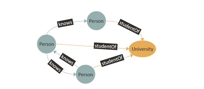
Here, student_network is the name of the graph. The graph has three vertices labeled Person and one vertex labeled University. There are six directed edges that connect the vertices. Three of them go from person to person vertices, and they have the label knows. Three others go from person to university vertices and are labeled studentOf. The person vertices have two properties, namely name for encoding the name of the person and dob for encoding the date of birth of the person. The university vertex has only a single property name for encoding the name of the university. The edges have no properties.

Example 2: Financial Transactions

An example graph with financial transactions is:

Here, financial_transactions is the name of the graph. The graph has three types of vertices. Vertices labeled Person or Company have a property name, while vertices labeled Account have a property number. There are edges labeled owner from accounts to persons as well as from accounts to companies, and there are edges labeled transaction from accounts to accounts. Note that only transaction edges have a property (amount) while other edges do not have any properties.

Creating a Property Graph

The CREATE PROPERTY GRAPH statement allows for creating a property graph from a set of existing database tables, while the DROP PROPERTY GRAPH statements allows for dropping a graph.

CREATE PROPERTY GRAPH

The CREATE PROPERTY GRAPH statement starts with a graph name and is followed by a non-empty set of vertex tables and an optional set of edge tables.

The syntax is:

CreatePropertyGraph  ::= 'CREATE' 'PROPERTY' 'GRAPH' GraphName
                         VertexTables
                         EdgeTables?

GraphName            ::= SchemaQualifiedName

SchemaQualifiedName  ::= SchemaIdentifierPart? Identifier

SchemaIdentifierPart ::= Identifier '.'

VertexTables         ::= 'VERTEX' 'TABLES' '(' VertexTable ( ',' VertexTable )* ')'

EdgeTables           ::= 'EDGE' 'TABLES' '(' EdgeTable ( ',' EdgeTable )* ')'

It is possible to have no edge tables such that the resulting graph only has vertices that are all disconnected from each other. However, it is not possible to have a graph with edge tables but no vertex tables.

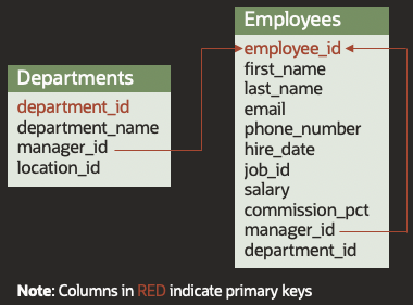
The following example shows a schema with a set of tables. Each table has a name and a list of columns, some of which form the primary key for the table (in red) while others form foreign keys that reference rows of other tables.

The following is a complete example of how a graph can be created from these tables:

CREATE PROPERTY GRAPH financial_transactions
  VERTEX TABLES (
    Persons LABEL Person PROPERTIES ( name ),
    Companies LABEL Company PROPERTIES ( name ),
    Accounts LABEL Account PROPERTIES ( number )
  )
  EDGE TABLES (
    Transactions
      SOURCE KEY ( from_account ) REFERENCES Accounts
      DESTINATION KEY ( to_account ) REFERENCES Accounts
      LABEL transaction PROPERTIES ( amount ),
    Accounts AS PersonOwner
      SOURCE KEY ( number ) REFERENCES Accounts
      DESTINATION Persons
      LABEL owner NO PROPERTIES,
    Accounts AS CompanyOwner
      SOURCE KEY ( number ) REFERENCES Accounts
      DESTINATION Companies
      LABEL owner NO PROPERTIES,
    Persons AS worksFor
      SOURCE KEY ( id ) REFERENCES Persons
      DESTINATION Companies
      NO PROPERTIES
  )

Above, financial_transactions is the name of the graph. The graph has three vertex tables: Persons, Companies and Accounts. The graph also has four edge tables: Transactions, PersonOwner, CompanyOwner and worksFor.

Underlying foreign keys are used to establish the connections between the two endpoints of the edges and the corresponding vertices. Note that the “source” of an edge is the vertex where the edge points from while the “destination” of an edge is the vertex where the edge point to.

If foreign keys cannot be used or are not present, the necessary keys can be defined as part of the CREATE PROPERTY GRAPH statement. Labels and properties can also be defined, all of which is explained in more detail in the next sections.

Vertex tables

A vertex table provides a vertex for each row of the underlying table.

The syntax is:

VertexTable              ::= TableName TableAlias? KeyClause? LabelAndPropertiesClause?

LabelAndPropertiesClause ::= LabelClause? PropertiesClause?

TableName                ::= SchemaQualifiedName

The table alias is required only if the underlying table is used as vertex table more than once, to provide a unique name for each table. It can be used for specifying a label for the vertices too.

The key of the vertex table uniquely identifies a row in the table. If a key is not explicitly specified then it defaults to the primary key of the underlying table. A key is always required so a primary key needs to exist if no key is specified. See the section on keys for more details.

The label clause provides a label for the vertices. If a label is not defined, the label defaults to the alias. Since the alias defaults to the name of the underlying table, if no alias is provided, the label defaults to the name of the underlying table. See the section on labels for details.

The properties clause defines the mapping from columns of the underlying table into properties of the vertices. See the section on properties for more details.

Edge tables

An edge table provides an edge for each row of the underlying table.

EdgeTable                      ::= TableName TableAlias? KeyClause?
                                   SourceVertexTable DestinationVertexTable
                                   LabelAndPropertiesClause?

SourceVertexTable              ::= 'SOURCE' ReferencedVertexTableKeyClause? TableName

DestinationVertexTable         ::= 'DESTINATION' ReferencedVertexTableKeyClause? TableName

ReferencedVertexTableKeyClause ::= KeyClause 'REFERENCES'

The table alias is required only if the underlying table is used as edge table more than once, to provide a unique name for each table. It can be used for specifying a label for the edges too.

The source vertex table and destination vertex table are mandatory for defining the two endpoints of the edge. A key is optional if there is a single foreign key from the edge table to the source or destination vertex table. If a key is not provided, it will default to the existing foreign key.

Take the following example from before:

CREATE PROPERTY GRAPH financial_transactions
  VERTEX TABLES (
    Persons LABEL Person PROPERTIES ( name ),
    Companies LABEL Company PROPERTIES ( name ),
    Accounts LABEL Account PROPERTIES ( number )
  )
  EDGE TABLES (
    Transactions
      SOURCE KEY ( from_account ) REFERENCES Accounts
      DESTINATION KEY ( to_account ) REFERENCES Accounts
      LABEL transaction PROPERTIES ( amount ),
    Accounts AS PersonOwner
      SOURCE KEY ( number ) REFERENCES Accounts
      DESTINATION Persons
      LABEL owner NO PROPERTIES,
    Accounts AS CompanyOwner
      SOURCE KEY ( number ) REFERENCES Accounts
      DESTINATION Companies
      LABEL owner NO PROPERTIES,
    Persons AS worksFor
      SOURCE KEY ( id ) REFERENCES Persons
      DESTINATION Companies
      NO PROPERTIES
  )

The key of the edge table uniquely identifies a row in the table. If a key is not explicitly specified (in case of all four edge tables above) then it defaults to the primary key of the underlying table. A key is always required so a primary key needs to exist if no key is specified. See the section on keys for more details.

In case of edge tables PersonOwner, CompanyOwner and worksFor, the destination vertex table is the same table as the edge table itself. This means that rows in the table are mapped into both vertices and edges. It is also possible that the source vertex table is the edge table itself or that both the source and destination tables are the edge table itself. This is explained in more detail in Source or destination is self.

Keys for the destinations of PersonOwner, CompanyOwner and worksFor are omitted because we can default to the existing foreign keys. Keys for their sources cannot be omitted because there exist no foreign key to default to (e.g. in case of PersonOwner there are zero foreign keys from Accounts to Accounts hence SOURCE KEY ( number ) REFERENCES Accounts needs to be specified). Furthermore, keys for the source and destination of Transactions cannot be omitted because two foreign keys exist between Transactions and Accounts so it is necessary to specify which one to use.

If a row in an edge table has a NULL value for any of its source key columns or its destination key columns then no edge is created. Note that in case of the Accounts table from the example, it is assumed that either the person_id or the company_id is NULL, so that each time the row is mapped into either a “company owner” or a “person owner” edge but never into two types of edges at once.

The label clause provides a label for the edges. If a label is not defined, the label defaults to the alias. Since the alias defaults to the name of the underlying table, if no alias is provided, the label defaults to the name of the underlying table. See the section on labels for details.

The properties clause defines the mapping from columns of the underlying table to properties of the edges. See the section on properties for more details

Table aliases

Vertex and edge tables can have aliases for uniquely naming the tables. If no alias is defined, then the alias defaults to the name of the underlying database table of the vertex or edge table.

The syntax is:

TableAlias ::= ( 'AS' )? Identifier

For example:

...
  EDGE TABLES ( Persons AS worksFor ... )
...

Above, the underlying table of the edge table is Persons, while the alias is worksFor.

All vertex and edge tables are required to have unique names. Therefore, if multiple vertex tables use the same underlying table, then at least one of them requires an alias. Similarly, if multiple edge tables use the same underlying table, then at least one of them requires an alias. The restriction does not apply across vertex and edge tables, so, there may exist a vertex table with the same name as an edge table, but there may not exist two vertex tables with the same name, or two edge tables with the same name.

If the alias is not provided then it defaults to the name of the underlying table. For example:

...
  VERTEX TABLES ( Person )
...

Above is equivalent to:

...
  VERTEX TABLES ( Person AS Person )
...

Finally, in addition to providing unique names for vertex and edge tables, the aliases can also serve as a means to provide labels for vertices and edges: if no label is defined then the label defaults to the table alias. Note that although table aliases are required to be unique, labels are not. In other words, multiple vertex tables and multiple edge tables can have the same label.

Keys

By default, existing primary and foreign keys of underlying tables are used to connect the end points of the edges to the appropriate vertices, but the following scenarios require manual specification of keys:

Multiple foreign keys exists between an edge table and its source vertex table or its destination vertex tables such that it would be ambiguous which foreign key to use.
Primary and/or foreign keys on underlying tables were not defined or the underlying tables are views which means that primary and foreign keys cannot be defined.

The syntax for keys is:

KeyClause  ::= '(' ColumnName ( ',' ColumnName )* ')'

ColumnName ::= Identifier

Take the example from before:

CREATE PROPERTY GRAPH financial_transactions
  VERTEX TABLES (
    ...
  )
  EDGE TABLES (
    Transactions
      SOURCE KEY ( from_account ) REFERENCES Accounts
      DESTINATION KEY ( to_account ) REFERENCES Accounts
      LABEL transaction PROPERTIES ( amount ),
    Accounts AS PersonOwner
      SOURCE KEY ( number ) REFERENCES Accounts
      DESTINATION Persons
      LABEL owner NO PROPERTIES,
    ...
  )

Above, a key is defined for the source and destination of Transactions because two foreign keys exist between Transactions and Accounts so it would be ambiguous which one to use without explicit specification. In case of PersonOwner, no foreign key exists between Accounts and Accounts so a key for the source (KEY ( number )) has to be explicitly specified. However, for the destination it is possible to omit the key and default to the existing foreign key between Accounts and Persons.

The keys for source and destination vertex tables consist of one or more columns of the underlying edge table that uniquely identify a vertex in the corresponding vertex table. If no key is defined for the vertex table, the key defaults to the underlying primary key, which is required to exist in such a case.

The following example has a schema that has no primary and foreign keys defined at all:

Note that above, we have the same schema as before, but this time the primary and foreign keys are missing.

Even though primary and foreign keys are missing, the graph can still be created by specifying the necessary keys in the CREATE PROPERTY GRAPH statement itself:

CREATE PROPERTY GRAPH financial_transactions
  VERTEX TABLES (
    Persons
      KEY ( id )
      LABEL Person
      PROPERTIES ( name ),
    Companies
      KEY ( id )
      LABEL Company
      PROPERTIES ( name ),
    Accounts
      KEY ( number )
      LABEL Account
      PROPERTIES ( number )
  )
  EDGE TABLES (
    Transactions
      KEY ( from_account, to_account, date )
      SOURCE KEY ( from_account ) REFERENCES Accounts
      DESTINATION KEY ( to_account ) REFERENCES Accounts
      LABEL transaction PROPERTIES ( amount ),
    Accounts AS PersonOwner
      KEY ( number )
      SOURCE KEY ( number ) REFERENCES Accounts
      DESTINATION KEY ( person_id ) REFERENCES Persons
      LABEL owner NO PROPERTIES,
    Accounts AS CompanyOwner
      KEY ( number )
      SOURCE KEY ( number ) REFERENCES Accounts
      DESTINATION KEY ( company_id ) REFERENCES Companies
      LABEL owner NO PROPERTIES,
  Persons AS worksFor
      KEY ( id )
      SOURCE KEY ( id ) REFERENCES Persons
      DESTINATION KEY ( company_id ) REFERENCES Companies
      NO PROPERTIES
  )

Above, keys were defined for each vertex table (e.g. KEY ( id )), edge table (e.g. KEY ( from_account, to_account, date )), source vertex table reference (e.g. KEY ( from_account )) and destination table reference (e.g. KEY ( to_account )).

Each vertex and edge table is required to have a key so that if a key is not explicitly specified then the underlying table needs to have a primary key defined.

Labels

In graphs created through CREATE PROPERTY GRAPH, each vertex has exactly one label and each edge has exactly one label. This restriction may be lifted in future PGQL version.

The syntax for labels is:

LabelClause ::= 'LABEL' Label

Label       ::= Identifier

The label clause is optional. If it is omitted, then the label defaults to the table alias. Note that also the table alias is optional and defaults to the table name. Thus, if no label is specified and no table alias is specified, then both the table alias and the label defaults to the table name.

For example:

...
  VERTEX TABLES ( Person )
...

Above is equivalent to:

...
  VERTEX TABLES ( Person AS Person )
...

Which is equivalent to:

...
  VERTEX TABLES ( Person AS Person LABEL Person )
...

Properties

By default, properties are all columns such that a vertex or edge property is created for each column of the underlying table. However, there are different ways to customize this behavior as described below.

The syntax is:

PropertiesClause ::=   PropertiesAreAllColumns
                     | PropertyExpressions
                     | NoProperties

Note that the properties clause is optional and if the clause is omitted then it defaults to PROPERTIES ARE ALL COLUMNS.

PROPERTIES ARE ALL COLUMNS

Although by default a property is created for each columns implicitly, this can also be made explicit through PROPERTIES ARE ALL COLUMNS.

The syntax is:

PropertiesAreAllColumns ::= 'PROPERTIES' AreKeyword? 'ALL' 'COLUMNS' ExceptColumns?

AreKeyword              ::= 'ARE'

An example is:

...
  VERTEX TABLES ( Person PROPERTIES ARE ALL COLUMNS )
...

Because of the default, the above is equivalent to:

...
  VERTEX TABLES ( Person )
...

PROPERTIES ARE ALL COLUMNS EXCEPT ( .. )

One can exclude columns by adding an EXCEPT clause. The columns that are excluded will not become properties while all the other columns do.

The syntax is:

ExceptColumns ::= 'EXCEPT' '(' ColumnReference ( ',' ColumnReference )* ')'

PROPERTIES ( .. )

Instead of excluding columns (see above), “property expressions” allow for specifying exactly which columns should be included. The property expressions also allow you to use a CAST expression to map the column into a property of a different data type.

The syntax is:

PropertyExpressions                ::= 'PROPERTIES' '(' PropertyExpression ( ',' PropertyExpression )* ')'

PropertyExpression                 ::= ColumnReferenceOrCastSpecification ( 'AS' PropertyName )?

ColumnReferenceOrCastSpecification ::=   ColumnReference
                                       | CastSpecification

PropertyName                       ::= Identifier

ColumnReference                    ::= Identifier

For example:

...
  VERTEX TABLES (
    Employees
      LABEL Employee
      PROPERTIES ( first_name ),
...

Above, even though table Employees may have many columns, only the column first_name is used as a property. The name of the property defaults to the name of the column: first_name.

If a different property name is desired then an alias can be used:

...
  VERTEX TABLES (
    Employees
      LABEL Employee
      PROPERTIES ( first_name AS firstName ),
...

Above, the column name first_name becomes a property with name firstName (notice the missing underscore character in the property name).

Property names may also be CAST expressions, which allows the values in the column to be converted into properties of a different data type.

For example:

...
  VERTEX TABLES (
    Employees
      LABEL Employee
      PROPERTIES ( CAST(salary AS INTEGER) AS salary ),
...

NO PROPERTIES

If no properties are desired for the vertices or edges, then one can use the NO PROPERTIES syntax:

NoProperties ::= 'NO' 'PROPERTIES'

An example of an edge table with no properties is:

...
  EDGE TABLES (
    ...
    Accounts AS PersonOwner
      SOURCE KEY ( number ) REFERENCES Accounts
      DESTINATION Persons
      LABEL owner NO PROPERTIES
    ...

Relation between labels and properties

Vertex tables that have the same label are required to have the same properties such that the properties have the same name and compatible data types. Similarly, edge tables that have the same label are required to have the same properties such that the properties have the same name and compatible data types.

Take the following example:

...
  VERTEX TABLES (
    /* ERROR: it is not allowed to have tables with the same labels but different properties */
    Country LABEL Place PROPERTIES ( country_name ),
    City LABEL Place PROPERTIES ( city_name )
  )
...

The statement above is illegal because both Country and City have label Place but their properties are inconsistent. To make this example work, the same property names have to be assigned:

...
  VERTEX TABLES (
    Country LABEL Place PROPERTIES ( country_name AS name ),
    City LABEL Place PROPERTIES ( city_name AS name )
  )
...

Source or destination is self

A source and/or a destination vertex table of an edge may be the edge table itself. In such a case, the underlying table provides both vertices and edges at the same time.

Take the following schema as example:

Here, both tables are clear candidates for vertex tables, but it is not immediately clear which are the edge tables corresponding to the “employee works for employee” and “department managed by employee” relationships.

These edge tables are in fact the Employees and Departments tables themselves.

The graph can be created as follows:

CREATE PROPERTY GRAPH hr_simplified
  VERTEX TABLES (
    employees LABEL employee
      PROPERTIES ARE ALL COLUMNS EXCEPT ( job_id, manager_id, department_id ),
    departments LABEL department
      PROPERTIES ( department_id, department_name )
  )
  EDGE TABLES (
    employees AS works_for
      SOURCE KEY ( employee_id ) REFERENCES employees
      DESTINATION KEY ( manager_id ) REFERENCES employees
      NO PROPERTIES,
    departments AS managed_by
      SOURCE KEY ( department_id ) REFERENCES departments
      DESTINATION employees
      NO PROPERTIES
  )

As you can see, the employee vertices are created from the employees table, but so are the works_for edges that represent the managers of employees. The source key is the primary key of the table, while the destination key corresponds to the foreign key. It is optional to simplify DESTINATION KEY ( manager_id ) REFERENCES employees to DESTINATION employees to make use of the existing foreign key. This is possible only because there exists exactly one foreign key between the employees table and itself. Do note that in this example, we cannot default the source vertex to the foreign key, so we need to explicitly specify it (KEY ( employee_id )).

Similarly, the department vertices are created from the departments table, but so are the managed_by edges that represent the managers of departments. The source of the edge table is again the table itself and therefore references the primary key. The destination, on the other hand, is the employees table. Here, because there exists a (single) foreign key between departments and employees, the destination key KEY ( manager_id ) was omitted to make it default to the foreign key.

Furthermore, even though the edges are embedded in the vertex tables, it is still the case that by default a property is created for each of the columns of the table. Therefore, we specify NO PROPERTIES for the edge tables as we already place the necessary properties on the vertex tables.

Example: HR schema

A more complex example is the Human Resources (HR) schema:

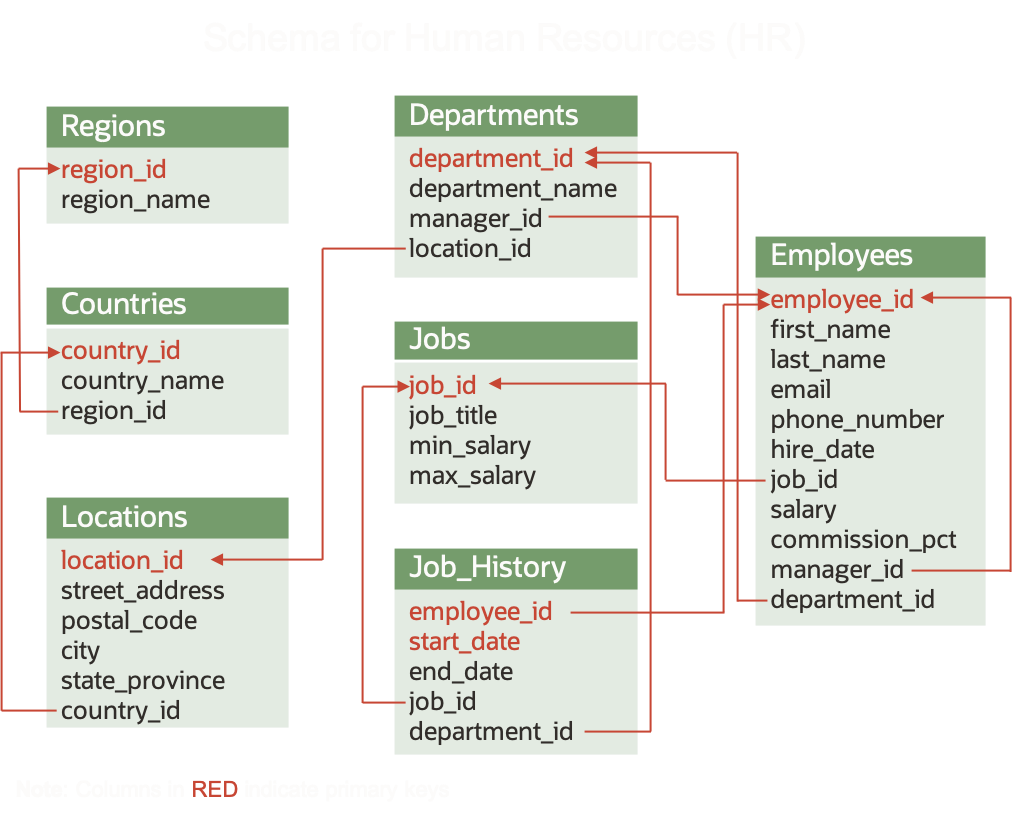
The following statement maps the schema into a graph:

CREATE PROPERTY GRAPH hr
  VERTEX TABLES (
    employees LABEL employee
      PROPERTIES ARE ALL COLUMNS EXCEPT ( job_id, manager_id, department_id ),
    departments LABEL department
      PROPERTIES ( department_id, department_name ),
    jobs LABEL job
      PROPERTIES ARE ALL COLUMNS,
    job_history
      PROPERTIES ( start_date, end_date ),
    locations LABEL location
      PROPERTIES ARE ALL COLUMNS EXCEPT ( country_id ),
    countries LABEL country
      PROPERTIES ARE ALL COLUMNS EXCEPT ( region_id ),
    regions LABEL region
  )
  EDGE TABLES (
    employees AS works_for
      SOURCE KEY ( employee_id ) REFERENCES employees
      DESTINATION KEY ( manager_id ) REFERENCES employees
      NO PROPERTIES,
    employees AS works_at
      SOURCE KEY ( employee_id ) REFERENCES employees
      DESTINATION departments
      NO PROPERTIES,
    employees AS works_as
      SOURCE KEY ( employee_id ) REFERENCES employees
      DESTINATION jobs
      NO PROPERTIES,
    departments AS managed_by
      SOURCE KEY ( department_id ) REFERENCES departments
      DESTINATION employees
      NO PROPERTIES,
    job_history AS for_employee
      SOURCE KEY ( employee_id, start_date ) REFERENCES job_history
      DESTINATION employees
      NO PROPERTIES,
    job_history AS for_department
      SOURCE KEY ( employee_id, start_date ) REFERENCES job_history
      DESTINATION departments
      NO PROPERTIES,
    job_history AS for_job
      SOURCE KEY ( employee_id, start_date ) REFERENCES job_history
      DESTINATION jobs
      NO PROPERTIES,
    departments AS department_located_in
      SOURCE KEY ( department_id ) REFERENCES departments
      DESTINATION locations
      LABEL located_in
      NO PROPERTIES,
    locations AS location_located_in
      SOURCE KEY ( location_id ) REFERENCES locations
      DESTINATION countries
      LABEL located_in
      NO PROPERTIES,
    countries AS country_located_in
      SOURCE KEY ( country_id ) REFERENCES countries
      DESTINATION regions
      LABEL located_in
      NO PROPERTIES
  )

In this example, all the edge tables have a source vertex table that is the edge table itself. This scenario was explained in more detail in Source or destination is self. Also note that the graph only has vertex properties, but no edge properties, which is typical for such a scenario.

After the graph is created it can be queried. For example, we may want to see an overview of the vertex and edge labels and their frequencies. Therefore, we first perform a SELECT query to create such an overview for the vertex labels:

  SELECT label(n) AS lbl, COUNT(*)
    FROM MATCH (n)
GROUP BY lbl
ORDER BY COUNT(*) DESC

+------------------------+
| lbl         | COUNT(*) |
+------------------------+
| EMPLOYEE    | 107      |
| DEPARTMENT  | 27       |
| COUNTRY     | 25       |
| LOCATION    | 23       |
| JOB         | 19       |
| JOB_HISTORY | 10       |
| REGION      | 4        |
+------------------------+

Note that above, labels are uppercased since unquoted identifiers were used in the CREATE PROPERTY GRAPH statement. Like in SQL, quoted identifiers can be used if such implicit upper casing of identifiers is not desired.

Then, we create an overview of labels of edges and labels of their source and destination vertices, again with frequencies for each combination:

  SELECT label(n) AS srcLbl, label(e) AS edgeLbl, label(m) AS dstLbl, COUNT(*)
    FROM MATCH (n) -[e]-> (m)
GROUP BY srcLbl, edgeLbl, dstLbl
ORDER BY COUNT(*) DESC

+--------------------------------------------------+
| srcLbl      | edgeLbl    | dstLbl     | COUNT(*) |
+--------------------------------------------------+
| EMPLOYEE    | WORKS_AS   | JOB        | 107      |
| EMPLOYEE    | WORKS_AT   | DEPARTMENT | 106      |
| EMPLOYEE    | WORKS_FOR  | EMPLOYEE   | 106      |
| DEPARTMENT  | LOCATED_IN | LOCATION   | 27       |
| COUNTRY     | LOCATED_IN | REGION     | 25       |
| LOCATION    | LOCATED_IN | COUNTRY    | 23       |
| DEPARTMENT  | MANAGED_BY | EMPLOYEE   | 11       |
| JOB_HISTORY | FOR        | JOB        | 10       |
| JOB_HISTORY | FOR        | EMPLOYEE   | 10       |
| JOB_HISTORY | FOR        | DEPARTMENT | 10       |
+--------------------------------------------------+

Multiple schemas

Vertex and edge tables of a graph can come from different database schemas. This can be achieved by qualifying the vertex and edge table names with a schema name.

For example:

CREATE PROPERTY GRAPH
  VERTEX TABLES (
    SocialNetwork.Person,
    HR.Employees LABEL Employee
  )
  EDGE TABLES (
    MySchema.SameAs
      SOURCE KEY ( firstName, lastName ) REFERENCES Person
      DESTINATION KEY ( first_name, last_name ) REFERENCES Employee
  )

Above, the vertex table Person is part of schema SocialNetwork, the vertex table Employee is part of schema HR and the edge table SameAs is part of schema MySchema.

Note that for the edge table, the source and destination vertex tables are referenced by table name without schema name (e.g. Person instead of SocialNetwork.Person). Also note that if no table aliases or labels are defined, then they default to the table name without the schema name.

DROP PROPERTY GRAPH

To drop a property graph use DROP PROPERTY GRAPH followed by the name of the graph to drop.

The syntax is:

DropPropertyGraph ::= 'DROP' 'PROPERTY' 'GRAPH' GraphName

For example:

DROP PROPERTY GRAPH financial_transactions

Graph Pattern Matching

Writing simple queries

This section is mostly example-based and is meant for beginning users.

Vertex patterns

The following query matches all the vertices with the label Person and retrieves their properties name and dob:

SELECT n.name, n.dob
  FROM MATCH (n:Person)

+-----------------------+
| name     | dob        |
+-----------------------+
| Riya     | 1995-03-20 |
| Kathrine | 1994-01-15 |
| Lee      | 1996-01-29 |
+-----------------------+

In the query above:

(n:Person) is a vertex pattern in which n is a variable name and :Person a label expression.
Variable names like n can be freely chosen by the user. The vertices that match the pattern are said to “bind to the variable”.
The label expression :Person specifies that we match only vertices that have the label Person.
n.name and n.dob are property references, accessing the properties name and dob of the vertex n respectively.

The query produces three results, which are returned as a table. The results are unordered.

Edge patterns

Edge patterns take the form of arrows like -[e]-> (match an outgoing edge) and <-[e]- (match an incoming edge).

For example:

SELECT a.name AS a, b.name AS b
  FROM MATCH (a:Person) -[e:knows]-> (b:Person)

+---------------------+
| a        | b        |
+---------------------+
| Kathrine | Riya     |
| Kathrine | Lee      |
| Lee      | Kathrine |
+---------------------+

In the above query:

-[e:knows]-> is an edge pattern in which e is a variable name and :knows a label expression.
The arrowhead -> specifies that the pattern matches edges that are outgoing from a and incoming to b.

Label expressions

More complex label expressions are supported through label disjunction. Furthermore, it is possible to omit a label expression.

Label disjunction

The bar operator (|) is a logical OR for specifying that a vertex or edge should match as long as it has at least one of the specified labels.

For example:

SELECT n.name, n.dob
  FROM MATCH (n:Person|University)

+--------------------------+
| name        | dob        |
+--------------------------+
| Riya        | 1995-03-20 |
| Kathrine    | 1994-01-15 |
| Lee         | 1996-01-29 |
| UC Berkeley | <null>     |
+--------------------------+

In the query above, (n:Person|University) matches vertices that have either the label Person or the label University. Note that in the result, there is a <null> value in the last row because the corresponding vertex does not have a property dob.

Omitting a label expression

Label expressions may be omitted so that the vertex or edge pattern will then match any vertex or edge.

For example:

SELECT n.name, n.dob
  FROM MATCH (n)

+--------------------------+
| name        | dob        |
+--------------------------+
| Riya        | 1995-03-20 |
| Kathrine    | 1994-01-15 |
| Lee         | 1996-01-29 |
| UC Berkeley | <null>     |
+--------------------------+

Note that the query gives the same results as before since both patterns (n) and (n:Person|University) match all the vertices in the example graph.

Filter predicates

Filter predicates provide a way to further restrict which vertices or edges may bind to patterns. A filter predicate is a boolean value expression and is placed in a WHERE clause.

For example, “find all persons that have a date of birth (dob) greater than 1995-01-01”:

SELECT n.name, n.dob
  FROM MATCH (n)
 WHERE n.dob > DATE '1995-01-01'

+---------------------+
| name   | dob        |
+---------------------+
| Riya   | 1995-03-20 |
| Lee    | 1996-01-29 |
+---------------------+

Above, the vertex pattern (n) initially matches all three Person vertices in the graph as well as the University vertex, since no label expression is specified. However, the filter predicate n.dob > DATE '1995-01-01' filters out Kathrine because her date of birth is before 1995-01-01. It also filters out UC Berkeley because the vertex does not have a property dob so that the reference n.dob returns null and since null > DATE '1995-01-01' is null (see three-valued logic) the final result is null, which has the same affect as false and thus this candidate solution gets filtered out.

Another example is to “find people that Kathrine knows and that are old than her”:

SELECT m.name AS name, m.dob AS dob
  FROM MATCH (n) -[e]-> (m)
 WHERE n.name = 'Kathrine' AND n.dob <= m.dob

+-------------------+
| name | dob        |
+-------------------+
| Riya | 1995-03-20 |
| Lee  | 1996-01-29 |
+-------------------+

Here, the pattern (n) -[e]-> (m) initially matches all the edges in the graph since it does not have any label expression. However, the filter expression n.name = 'Kathrine' AND n.dob <= m.dob specifies that the source of the edge has a property name with the value Kathrine and that both the source and destination of the edge have properties dob such that the value for the source is smaller than or equal to the value for the destination. Only two out of six edges satisfy this filter predicate.

More complex patterns

More complex patterns are formed either by forming longer path patterns that consist of multiple edge patterns, or by specifying multiple comma-separated path patterns that share one or more vertex variables.

For example, “find people that Lee knows and that are a student at the same university as Lee”:

SELECT p2.name AS friend, u.name AS university
  FROM MATCH (u:University) <-[:studentOf]- (p1:Person) -[:knows]-> (p2:Person) -[:studentOf]-> (u)
 WHERE p1.name = 'Lee'

+------------------------+
| friend   | university  |
+------------------------+
| Kathrine | UC Berkeley |
+------------------------+

Above, in the MATCH clause there is only one path pattern that consists of four vertex patterns and three edge patterns. Note that the first and last vertex pattern both have the variable u. This means that they are the same variable rather than two different variables. Label expressions may be specified for neither, one, or both of the vertex patterns such that if there are multiple label expressions specified then they are simply evaluated in conjunction such that all expressions need to satisfy for a vertex to bind to the variable.

The same query as above may be expressed through multiple comma-separated path patterns, like this:

SELECT p2.name AS friend, u.name AS university
  FROM MATCH (p1:Person) -[:knows]-> (p2:Person)
     , MATCH (p1) -[:studentOf]-> (u:University)
     , MATCH (p2) -[:studentOf]-> (u)
 WHERE p1.name = 'Lee'

+------------------------+
| friend   | university  |
+------------------------+
| Kathrine | UC Berkeley |
+------------------------+

Here again, both occurrences of u are the same variable, as well as both occurrences of p1 and both occurrences of p2.

Binding an element multiple times

In a single solution it is allowed for a vertex or an edge to be bound to multiple variables at the same time.

For example, “find friends of friends of Lee” (friendship being defined by the presence of a ‘knows’ edge):

SELECT p1.name AS p1, p2.name AS p2, p3.name AS p3
  FROM MATCH (p1:Person) -[:knows]-> (p2:Person) -[:knows]-> (p3:Person)
 WHERE p1.name = 'Lee'

+-----------------------+
| p1  | p2       | p3   |
+-----------------------+
| Lee | Kathrine | Riya |
| Lee | Kathrine | Lee  |
+-----------------------+

Above, in the second solution, Lee is bound to both the variable p1 and the variable p3. This solution is obtained since we can hop from Lee to Kathrine via the edge that is outgoing from Lee, and then we can hop back from Kathrine to Lee via the edge that is incoming to Lee.

If such binding of vertices to multiple variables is not desired, one can use either non-equality constraints or the ALL_DIFFERENT predicate.

For example, the predicate p1 <> p3 in the query below adds the restriction that Lee, which has to bind to variable p1, cannot also bind to variable p3:

SELECT p1.name AS p1, p2.name AS p2, p3.name AS p3
  FROM MATCH (p1:Person) -[:knows]-> (p2:Person) -[:knows]-> (p3:Person)
 WHERE p1.name = 'Lee' AND p1 <> p3

+-----------------------+
| p1  | p2       | p3   |
+-----------------------+
| Lee | Kathrine | Riya |
+-----------------------+

An alternative is to use the ALL_DIFFERENT predicate, which can take any number of vertices or edges as input and specifies non-equality between all of them:

SELECT p1.name AS p1, p2.name AS p2, p3.name AS p3
  FROM MATCH (p1:Person) -[:knows]-> (p2:Person) -[:knows]-> (p3:Person)
 WHERE p1.name = 'Lee' AND ALL_DIFFERENT(p1, p3)

+-----------------------+
| p1  | p2       | p3   |
+-----------------------+
| Lee | Kathrine | Riya |
+-----------------------+

Besides vertices binding to multiple variables, it is also possible for edges to bind to multiple variables.

For example, “find two people that both know Riya”:

SELECT p1.name AS p1, p2.name AS p2, e1 = e2
  FROM MATCH (p1:Person) -[e1:knows]-> (riya:Person)
     , MATCH (p2:Person) -[e2:knows]-> (riya)
 WHERE riya.name = 'Riya'

+-------------------------------+
| p1       | p2       | e1 = e2 |
+-------------------------------+
| Kathrine | Kathrine | true    |
+-------------------------------+

Above, the only solution has Kathrine bound to both variables p1 and p2 and the single edge between Kathrine and Riya is bound to both e1 and e2, which is why e1 = e2 in the SELECT clause returns true.

Again, if such bindings are not desired then one should add constraints like e1 <> e2 or ALL_DIFFERENT(e1, e2) to the WHERE clause.

Matching edges in any direction

Any-directed edge patterns match edges in the graph no matter if they are incoming or outgoing.

An example query with two any-directed edge patterns is:

SELECT *
  FROM MATCH (n) -[e1]- (m) -[e2]- (o)

Note that in case there are both incoming and outgoing data edges between two data vertices, there will be separate result bindings for each of the edges.

Any-directed edge patterns may also be used inside path pattern macros:

  PATH two_hops AS () -[e1]- () -[e2]- ()
SELECT *
  FROM MATCH (n) -/:two_hops*/-> (m)

The above query will return all pairs of vertices n and m that are reachable via a multiple of two edges, each edge being either an incoming or an outgoing edge.

Main query structure

The previous section on writing simple queries provided a basic introduction to graph pattern matching. The rest of this document introduces the different functionalities in more detail.

The following is the syntax of the main query structure:

PgqlStatement   ::=   CreatePropertyGraph
                    | DropPropertyGraph
                    | Query

Query           ::=   SelectQuery
                    | ModifyQuery

SelectQuery     ::= PathPatternMacros?
                    SelectClause
                    FromClause
                    WhereClause?
                    GroupByClause?
                    HavingClause?
                    OrderByClause?
                    LimitOffsetClauses?

Details of the different clauses of a query can be found in the following sections:

The path pattern macros allow for specifying complex reachability queries.
The SELECT clause specifies what should be returned.
The FROM clause defines the graph pattern that is to be matched.
The WHERE clause specifies filters.
The GROUP BY clause allows for creating groups of results.
The HAVING clause allows for filtering entire groups of results.
The ORDER BY clause allows for sorting of results.
The LIMIT and OFFSET clauses allow for pagination of results.

SELECT

In a PGQL query, the SELECT clause defines the data entities to be returned in the result. In other words, the select clause defines the columns of the result table.

The following explains the syntactic structure of SELECT clause.

SelectClause ::= 'SELECT' 'DISTINCT'? ExpAsVar ( ',' ExpAsVar )*
               | 'SELECT' '*'

ExpAsVar     ::= ValueExpression ( 'AS' VariableName )?

A SELECT clause consists of the keyword SELECT followed by either an optional DISTINCT modifier and comma-separated sequence of ExpAsVar (“expression as variable”) elements, or, a special character star *. An ExpAsVar consists of:

A ValueExpression.
An optional VariableName, specified by appending the keyword AS and the name of the variable.

Consider the following example:

SELECT n, m, n.age AS age
  FROM MATCH (n:Person) -[e:friend_of]-> (m:Person)

Per each matched subgraph, the query returns two vertices n and m and the value for property age of vertex n. Note that edge e is omitted from the result even though it is used for describing the pattern.

The DISTINCT modifier allows for filtering out duplicate results. The operation applies to an entire result row, such that rows are only considered duplicates of each other if they contain the same set of values.

Assigning variable name to Select Expression

It is possible to assign a variable name to any of the selection expression, by appending the keyword AS and a variable name. The variable name is used as the column name of the result set. In addition, the variable name can be later used in the ORDER BY clause. See the related section later in this document.

  SELECT n.age * 2 - 1 AS pivot, n.name, n
    FROM MATCH (n:Person) -> (m:Car)
ORDER BY pivot

SELECT *

SELECT * is a special SELECT clause. The semantic of SELECT * is to select all the variables in the graph pattern.

Consider the following query:

SELECT *
  FROM MATCH (n:Person) -> (m) -> (w)
     , MATCH (n) -> (w) -> (m)

This query is semantically equivalent to:

SELECT n, m, w
  FROM MATCH (n:Person) -> (m) -> (w)
     , MATCH (n) -> (w) -> (m)

SELECT * is not allowed when the graph pattern has zero variables. This is the case when all the vertices and edges in the pattern are anonymous (e.g. MATCH () -> (:Person)). Furthermore, SELECT * in combination with GROUP BY is not allowed.

FROM

In a PGQL query, the FROM clause defines the graph pattern to be matched.

Syntactically, a FROM clause is composed of the keyword FROM followed by a comma-separated sequence of MATCH clauses, each defining a path pattern:

FromClause             ::= 'FROM' MatchClause ( ',' MatchClause )*

MATCH

MatchClause            ::= 'MATCH' ( PathPattern | GraphPattern ) OnClause?

GraphPattern           ::= '(' PathPattern ( ',' PathPattern )* ')'

PathPattern            ::=   SimplePathPattern
                           | ShortestPathPattern
                           | TopKShortestPathPattern
                           | CheapestPathPattern
                           | TopKCheapestPathPattern


SimplePathPattern      ::= VertexPattern ( PathPrimary VertexPattern )*

VertexPattern          ::= '(' VariableSpecification ')'

PathPrimary            ::=   EdgePattern
                           | ReachabilityPathExpression

EdgePattern            ::=   OutgoingEdgePattern
                           | IncomingEdgePattern
                           | AnyDirectedEdgePattern

OutgoingEdgePattern    ::=   '->'
                           | '-[' VariableSpecification ']->'

IncomingEdgePattern    ::=   '<-'
                           | '<-[' VariableSpecification ']-'

AnyDirectedEdgePattern ::=   '-'
                           | '-[' VariableSpecification ']-'

VariableSpecification  ::= VariableName? LabelPredicate?

VariableName           ::= Identifier

A path pattern that describes a partial topology of the subgraph pattern. In other words, a topology constraint describes some connectivity relationships between vertices and edges in the pattern, whereas the whole topology of the pattern is described with one or multiple topology constraints.

A topology constraint is composed of one or more vertices and relations, where a relation is either an edge or a path. In a query, each vertex or edge is (optionally) associated with a variable, which is a symbolic name to reference the vertex or edge in other clauses. For example, consider the following topology constraint:

(n) -[e]-> (m)

The above example defines two vertices (with variable names n and m), and an edge (with variable name e) between them. Also the edge is directed such that the edge e is an outgoing edge from vertex n.

More specifically, a vertex term is written as a variable name inside a pair of parenthesis (). An edge term is written as a variable name inside a square bracket [] with two dashes and an inequality symbol attached to it – which makes it look like an arrow drawn in ASCII art. An edge term is always connected with two vertex terms as for the source and destination vertex of the edge; the source vertex is located at the tail of the ASCII arrow and the destination at the head of the ASCII arrow.

There can be multiple path patterns in the FROM clause of a PGQL query. Semantically, all constraints are conjunctive – that is, each matched result should satisfy every constraint in the FROM clause.

ON clause

The ON clause is an optional clause that belongs to the MATCH clause and specifies the name of the graph to match the pattern on.

The syntax is:

OnClause   ::= 'ON' GraphName

For example:

  SELECT p.first_name, p.last_name
    FROM MATCH (p:Person) ON my_graph
ORDER BY p.first_name, p.last_name

Above, the pattern (p:Person) is matched on graph my_graph.

Default graphs

The ON clauses may be omitted if a “default graph” has been provided. PGQL itself does not (yet) provide syntax for specifying a default graph, but Java APIs for invoking PGQL queries typically provide mechanisms for it:

Oracle’s in-memory analytics engine PGX has the API PgxGraph.queryPgql("SELECT ...") such that the default graph corresponds to PgxGraph.getName() such that ON clauses can be omitted from queries.
Oracle’s PGQL-on-RDBMS provides the API PgqlConnection.setGraph("myGraph") for setting the default graph such that the ON clauses can be omitted from queries.

If a default graph is provided then the ON clause can be omitted:

  SELECT p.first_name, p.last_name
    FROM MATCH (p:Person)
ORDER BY p.first_name, p.last_name

Querying multiple graphs

Although each MATCH clause can have its own ON clause, PGQL 1.3 does not support querying of multiple graphs in a single query. Therefore, it is not possible for two MATCH clauses to have ON clauses with different graph names.

Repeated variables

There can be multiple topology constraints in the FROM clause of a PGQL query. In such a case, vertex terms that have the same variable name correspond to the same vertex entity. For example, consider the following two lines of topology constraints:

SELECT *
 FROM MATCH (n) -[e1]-> (m1)
    , MATCH (n) -[e2]-> (m2)

Here, the vertex term (n) in the first constraint indeed refers to the same vertex as the vertex term (n) in the second constraint. It is an error, however, if two edge terms have the same variable name, or, if the same variable name is assigned to an edge term as well as to a vertex term in a single query.

Alternatives for specifying graph patterns

There are various ways in which a particular graph pattern can be specified.

First, a single path pattern can be written as a chain of edge terms such that two consecutive edge terms share the common vertex term in between. For example:

SELECT *
  FROM MATCH (n1) -[e1]-> (n2) -[e2]-> (n3) -[e3]-> (n4)

The above graph pattern is equivalent to the graph pattern specified by the following set of comma-separate path patterns:

SELECT *
  FROM MATCH (n1) -[e1]-> (n2)
     , MATCH (n2) -[e2]-> (n3)
     , MATCH (n3) -[e3]-> (n4)

Second, it is allowed to reverse the direction of an edge in the pattern, i.e. right-to-left instead of left-to-right. Therefore, the following is a valid graph pattern:

SELECT *
  FROM MATCH (n1) -[e1]-> (n2) <-[e2]- (n3)

Please mind the edge directions in the above query – vertex n2 is a common outgoing neighbor of both vertex n1 and vertex n3.

Third, it is allowed to ommitg variable names if the particular vertex or edge does not need to be referenced in any of the other clauses (e.g. SELECT or ORDER BY). When the variable name is omitted, the vertex or edge is an “anonymous” vertex or edge.

Syntactically, for vertices, this result in an empty pair of parenthesis. In case of edges, the whole square bracket is omitted in addition to the variable name.

The following table summarizes these short cuts.

syntax form	example
basic form	`(n) -[e]-> (m)`
omit variable name of the source vertex	`() -[e]-> (m)`
omit variable name of the destination vertex	`(n) -[e]-> ()`
omit variable names in both vertices	`() -[e]-> ()`
omit variable name in edge	`(n) -> (m)`

Disconnected graph patterns

In the case the MATCH clause contains two or more disconnected graph patterns (i.e. groups of vertices and relations that are not connected to each other), the different groups are matched independently and the final result is produced by taking the Cartesian product of the result sets of the different groups. The following is an example:

SELECT *
  FROM MATCH (n1) -> (m1)
     , MATCH (n2) -> (m2)

Here, vertices n2 and m2 are not connected to vertices n1 and m1, resulting in a Cartesian product.

Label predicates

In the property graph model, vertices and edge may have labels, which are arbitrary (character) strings. Typically, labels are used to encode types of entities. For example, a graph may contain a set of vertices with the label Person, a set of vertices with the label Movie, and, a set of edges with the label likes. A label predicate specifies that a vertex or edge only matches if it has ony of the specified labels. The syntax for specifying a label predicate is through a (:) followed by one or more labels that are separate by a vertical bar (|).

This is explained by the following grammar constructs:

LabelPredicate ::= ':' Label ( '|' Label )*```

Take the following example:

SELECT *
  FROM MATCH (x:Person) -[e:likes|knows]-> (y:Person)

Here, we specify that vertices x and y have the label Person and that the edge e has the label likes or the label knows.

A label predicate can be specified even when a variable is omitted. For example:

SELECT *
  FROM MATCH (:Person) -[:likes|knows]-> (:Person)

There are also built-in functions available for labels:

label(element) returns the label of a vertex or edge in the case the vertex/edge has only a single label
labels(element) returns the set of labels of a vertex or edge in the case the vertex/edge has multiple labels.
has_label(element, string) returns true if the vertex or edge (first argument) has the specified label (second argument).

WHERE

Filters are applied after pattern matching to remove certain solutions. A filter takes the form of a boolean value expression which typically involves certain property values of the vertices and edges in the graph pattern.

The syntax is:

WhereClause ::= 'WHERE' ValueExpression

For example:

SELECT y.name
  FROM MATCH (x) -> (y)
 WHERE x.name = 'Jake'
   AND y.age > 25

Here, the first filter describes that the vertex x has a property name and its value is Jake. Similarly, the second filter describes that the vertex y has a property age and its value is larger than 25. Here, in the filter, the dot (.) operator is used for property access. For the detailed syntax and semantic of expressions, see Functions and Expressions.

Note that the ordering of constraints does not have an affect on the result, such that query from the previous example is equivalent to:

SELECT y.name
 FROM MATCH (x) -> (y)
WHERE y.age > 25
  AND x.name = 'Jake'

Grouping and Aggregation

GROUP BY

GROUP BY allows for grouping of solutions and is typically used in combination with aggregates like MIN and MAX to compute aggregations over groups of solutions.

The following explains the syntactic structure of the GROUP BY clause:

GroupByClause ::= 'GROUP' 'BY' ExpAsVar ( ',' ExpAsVar )*

The GROUP BY clause starts with the keywords GROUP BY and is followed by a comma-separated list of value expressions that can be of any type.

Consider the following query:

  SELECT n.first_name, COUNT(*), AVG(n.age)
    FROM MATCH (n:Person)
GROUP BY n.first_name

Matches are grouped by their values for n.first_name. For each group, the query selects n.first_name (i.e. the group key), the number of solutions in the group (i.e. COUNT(*)), and the average value of the property age for vertex n (i.e. AVG(n.age)).

Multiple Terms in GROUP BY

It is possible that the GROUP BY clause consists of multiple terms. In such a case, matches are grouped together only if they hold the same result for each of the group expressions.

Consider the following query:

  SELECT n.first_name, n.last_name, COUNT(*)
    FROM MATCH (n:Person)
GROUP BY n.first_name, n.last_name

Matches will be grouped together only if they hold the same values for n.first_name and the same values for n.last_name.

Aliases in GROUP BY

Each expression in GROUP BY can have an alias (e.g. GROUP BY n.prop AS myAlias). The alias can be referenced from the HAVING, ORDER BY and SELECT clauses so that repeated specification of the same expression can be avoided.

Note, however, that GROUP BY can also reference aliases from SELECT but it is not allowed to create a circular dependency such that an expression in the SELECT references an expression in the GROUP BY that in its turn references that same expression in the SELECT.

GROUP BY and NULL values

The group for which all the group keys are null is a valid group and takes part in further query processing.

To filter out such a group, use a HAVING clause (see HAVING), for example:

  SELECT n.prop1, n.prop2, COUNT(*)
    FROM MATCH (n)
GROUP BY n.prop1, n.prop2
  HAVING n.prop1 IS NOT NULL AND n.prop2 IS NOT NULL

Repetition of Group Expression in Select or Order Expression

Group expressions may be repeated in select or order expressions.

Consider the following query:

  SELECT n.age, COUNT(*)
    FROM MATCH (n)
GROUP BY n.age
ORDER BY n.age

Here, the group expression n.age is repeated in the SELECT and ORDER BY.

Aggregation

Aggregates COUNT, MIN, MAX, AVG and SUM can aggregate over groups of solutions.

The syntax is:

Aggregation      ::=   CountAggregation
                     | MinAggregation
                     | MaxAggregation
                     | AvgAggregation
                     | SumAggregation
                     | ArrayAggregation

CountAggregation ::=   'COUNT' '(' '*' ')'
                     | 'COUNT' '(' 'DISTINCT'? ValueExpression ')'

MinAggregation   ::= 'MIN' '(' 'DISTINCT'? ValueExpression ')'

MaxAggregation   ::= 'MAX' '(' 'DISTINCT'? ValueExpression ')'

AvgAggregation   ::= 'AVG' '(' 'DISTINCT'? ValueExpression ')'

SumAggregation   ::= 'SUM' '(' 'DISTINCT'? ValueExpression ')'

ArrayAggregation ::= 'ARRAY_AGG' '(' 'DISTINCT'? ValueExpression ')'

Syntactically, an aggregation takes the form of aggregate followed by an optional DISTINCT modifier and a ValueExpression.

The following table gives an overview of the different aggregates and their supported input types.

aggregate operator	semantic	required input type
`COUNT`	counts the number of times the given expression has a bound (i.e. is not null).	any type, including vertex and edge
`MIN`	takes the minimum of the values for the given expression.	numeric, string, boolean, date, time [with time zone], or, timestamp [with time zone]
`MAX`	takes the maximum of the values for the given expression.	numeric, string, boolean, date, time [with time zone], or, timestamp [with time zone]
`SUM`	sums over the values for the given expression.	numeric
`AVG`	takes the average of the values for the given expression.	numeric
`ARRAY_AGG`	constructs an array/list of the values for the given expression.	numeric, string, boolean, date, time [with time zone], or, timestamp [with time zone]

All aggregate functions ignore nulls. COUNT never returns null, but instead returns zero if all input values to the aggregate function are null. For all the remaining aggregate functions, if there are no inputs or all input values to the aggregate function are null, then the function returns null.

For example, the average of 2, 4 and null is 3, while the average of null and null is null. The count of 2, 4 and null is 2 (there are two non-null values), while the count of null and null is 0.

Aggregation with GROUP BY

If a GROUP BY is specified, aggregations are applied to each individual group of solutions.

For example:

  SELECT AVG(m.salary)
    FROM MATCH (m:Person)
GROUP BY m.age

Here, we group people by their age and compute the average salary for each such a group.

Aggregation without GROUP BY

If no GROUP BY is specified, aggregations are applied to the entire set of solutions.

For example:

SELECT AVG(m.salary)
  FROM MATCH (m:Person)

Here, we aggregate over the entire set of vertices with label Person, to compute the average salary.

COUNT(*)

COUNT(*) is a special construct that simply counts the number of solutions without evaluating an expression.

For example:

SELECT COUNT(*)
  FROM MATCH (m:Person)

DISTINCT in aggregation

The DISTINCT modifier specifies that duplicate values should be removed before performing aggregation.

For example:

SELECT AVG(DISTINCT m.age)
  FROM MATCH (m:Person)

Here, we aggregate only over distinct m.age values.

HAVING

The HAVING clause is an optional clause that can be placed after a GROUP BY clause to filter out particular groups of solutions.

The syntax is:

HavingClause ::= 'HAVING' ValueExpression

The value expression needs to be a boolean expression.

For example:

  SELECT n.name
    FROM MATCH (n) -[:has_friend]-> (m)
GROUP BY n
  HAVING COUNT(m) > 10

This query returns the names of people who have more than 10 friends.

Sorting and Row Limiting

ORDER BY

When there are multiple matched subgraph instances to a given query, in general, the ordering between those instances are not defined; the query execution engine can present the result in any order. Still, the user can specify the ordering between the answers in the result using ORDER BY clause.

The following explains the syntactic structure of ORDER BY clause.

OrderByClause ::= 'ORDER' 'BY' OrderTerm ( ',' OrderTerm )*

OrderTerm     ::= ValueExpression ( 'ASC' | 'DESC' )?

The ORDER BY clause starts with the keywords ORDER BY and is followed by comma separated list of order terms. An order term consists of the following parts:

An expression.
An optional ASC or DESC decoration to specify that ordering should be ascending or descending.
- If no keyword is given, the default is ascending order.

The following is an example in which the results are ordered by property access n.age in ascending order:

  SELECT n.name
    FROM MATCH (n:Person)
ORDER BY n.age ASC

Data types for ORDER BY

A partial ordering for the different data types is defined as follows:

Numeric values are ordered from small to large.
String values are ordered lexicographically.
Boolean values are ordered such that false comes before true.
Datetime values (i.e. dates, times, or timestamps) are ordered such that earlier points in time come before later points in time.

Vertices and edges cannot be ordered directly.

Multiple expressions in ORDER BY

An ORDER BY may contain more than one expression, in which case the expresisons are evaluated from left to right. That is, (n+1)th ordering term is used only for the tie-break rule for n-th ordering term. Note that different expressions can have different ascending or descending decorators.

  SELECT f.name
    FROM MATCH (f:Person)
ORDER BY f.age ASC, f.salary DESC

LIMIT and OFFSET

The LIMIT puts an upper bound on the number of solutions returned, whereas the OFFSET specifies the start of the first solution that should be returned.

The following explains the syntactic structure for the LIMIT and OFFSET clauses:

LimitOffsetClauses ::=   'LIMIT' LimitOffsetValue ( 'OFFSET' LimitOffsetValue )?
                       | 'OFFSET' LimitOffsetValue ( 'LIMIT' LimitOffsetValue )?

LimitOffsetValue   ::=   UNSIGNED_INTEGER
                       | BindVariable

The LIMIT clause starts with the keyword LIMIT and is followed by an integer that defines the limit. Similarly, the OFFSET clause starts with the keyword OFFSET and is followed by an integer that defines the offset. Furthermore: The LIMIT and OFFSET clauses can be defined in either order. The limit and offset may not be negatives. The following semantics hold for the LIMIT and OFFSET clauses: The OFFSET clause is always applied first, even if the LIMIT clause is placed before the OFFSET clause inside the query. An OFFSET of zero has no effect and gives the same result as if the OFFSET clause was omitted. If the number of actual solutions after OFFSET is applied is greater than the limit, then at most the limit number of solutions will be returned.

In the following query, the first 5 intermediate solutions are pruned from the result (i.e. OFFSET 5). The next 10 intermediate solutions are returned and become final solutions of the query (i.e. LIMIT 10).

SELECT n
  FROM MATCH (n)
 LIMIT 10
OFFSET 5

Variable-Length Paths

Graph Pattern Matching introduced how “fixed-length” patterns can be matched. Fixed-length patterns match a fixed number of vertices and edges such that every solution (every row) has the same number of vertices and edges.

However, through the use of quantifiers (introduced below) it is is possible to match “variable-length” paths such as shortest paths. Variable-length path patterns match a variable number of vertices and edges such that different solutions (different rows) potentially have different numbers of vertices and edges.

Quantifiers

Quantifiers allow for matching variable-length paths by specifying lower and upper limits on the number of times a pattern is allowed to match.

The syntax is:

GraphPatternQuantifier     ::=   ZeroOrMore
                               | OneOrMore
                               | Optional
                               | ExactlyN
                               | NOrMore
                               | BetweenNAndM
                               | BetweenZeroAndM

ZeroOrMore                 ::= '*'

OneOrMore                  ::= '+'

Optional                   ::= '?'

ExactlyN                   ::= '{' UNSIGNED_INTEGER '}'

NOrMore                    ::= '{' UNSIGNED_INTEGER ',' '}'

BetweenNAndM               ::= '{' UNSIGNED_INTEGER ',' UNSIGNED_INTEGER '}'

BetweenZeroAndM            ::= '{' ',' UNSIGNED_INTEGER '}'

The meaning of the different quantifiers is:

quantifier	meaning	matches
*	zero (0) or more	a path that connects the source and destination of the path by zero or more matches of a given pattern
+	one (1) or more	a path that connects the source and destination of the path by one or more matches of a given pattern
?	zero or one (1), i.e. “optional”	a path that connects the source and destination of the path by zero or one matches of a given pattern
{ n }	exactly n	a path that connects the source and destination of the path by exactly n matches of a given pattern
{ n, }	n or more	a path that connects the source and destination of the path by at least n matches of a given pattern
{ n, m }	between n and m (inclusive)	a path that connects the source and destination of the path by at least n and at most m (inclusive) matches of a given pattern
{ , m }	between zero (0) and m (inclusive)	a path that connects the source and destination of the path by at least 0 and at most m (inclusive) matches of a given pattern

All paths are considered, even the ones that contain a vertex or edge multiple times. In other words, cycles are permitted.

An example is:

SELECT a.number AS a,
       b.number AS b,
       COUNT(e) AS pathLength,
       ARRAY_AGG(e.amount) AS amounts
  FROM MATCH SHORTEST ( (a:Account) -[e:transaction]->* (b:Account) )
 WHERE a.number = 10039 AND b.number = 2090

+------------------------------------------------------+
| a     | b    | pathLength | amounts                  |
+------------------------------------------------------+
| 10039 | 2090 | 3          | [1000.0, 1500.3, 9999.5] |
+------------------------------------------------------+

Above, we use the quantifier * to find a shortest path from account 10039 to account 2090, following only transaction edges. Shortest path finding is explained in more detail in Shortest Path. COUNT(e) and ARRAY_AGG(e.amount) are horizontal aggregations which are explained in Horizontal Aggregation.

Reachability

In graph reachability we test for the existence of paths (true/false) between pairs of vertices. PGQL uses forward slashes (-/ and /->) instead of square brackets (-[ and ]->) to indicate reachability semantic.

The syntax is:

ReachabilityPathExpression ::=   OutgoingPathPattern
                               | IncomingPathPattern

OutgoingPathPattern        ::= '-/' PathSpecification '/->'

IncomingPathPattern        ::= '<-/' PathSpecification '/-'

PathSpecification          ::=   LabelPredicate
                               | PathPredicate

PathPredicate              ::= ':' Label GraphPatternQuantifier?

For example:

SELECT c.name
  FROM MATCH (c:Class) -/:subclass_of*/-> (arrayList:Class)
 WHERE arrayList.name = 'ArrayList'

Here, we find all classes that are a subclass of 'ArrayList'. The regular path pattern subclass_of* matches a path consisting of zero or more edges with the label subclass_of. Because the pattern may match a path with zero edges, the two query vertices can be bound to the same data vertex if the data vertex satisfies the constraints specified in both source and destination vertices (i.e. the vertex has a label Class and a property name with a value ArrayList).

Examples with various quantifiers

Zero or more

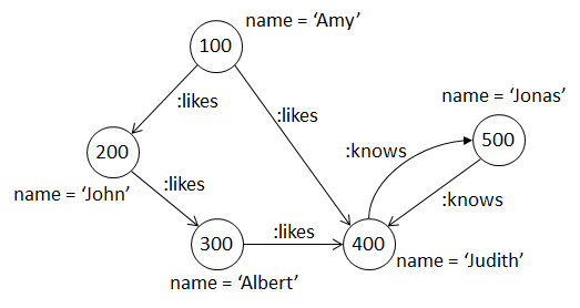
The following example finds all vertices y that can be reached from Amy by following zero or more likes edges.

SELECT y.name
  FROM MATCH (x:Person) -/:likes*/-> (y)
 WHERE x.name = 'Amy'

+--------+
| y.name |
+--------+
| Amy    |
| John   |
| Albert |
| Judith |
+--------+

Note that here, Amy is returned since Amy connects to Amy by following zero likes edges. In other words, there exists an empty path for the vertex pair. For Judith, there exist two paths (100 -> 200 -> 300 -> 400 and 100 -> 400). However, Judith is still only returned once since the semantic of -/ .. /-> is to test for the existence of paths between pairs of vertices (i.e. “reachability”), so there is only at most one result per pair of vertices.

One or more

The following example finds all people that can be reached from Amy by following one or more likes edges.

SELECT y.name
  FROM MATCH (x:Person) -/:likes+/-> (y)
 WHERE x.name = 'Amy'

+--------+
| y.name |
+--------+
| John   |
| Albert |
| Judith |
+--------+

This time, Amy is not returned since there does not exist a path that connects Amy to Amy that has a length greater than zero.

The following example finds all people that can be reached from Judith by following one or more knows edges:

SELECT y.name
  FROM MATCH (x:Person) -/:knows+/-> (y)
 WHERE x.name = 'Judith'

+--------+
| y.name |
+--------+
| Jonas  |
| Judith |
+--------+

Here, in addition to Jonas, Judith is returned since there exist paths from Judith back to Judith that has a length greater than zero. Examples of such paths are 400 -> 500 -> 400 and 400 -> 500 -> 400 -> 500 -> 400.

Optional

The following example finds all people that can be reached from Judith by following zero or one knows edges.

SELECT y.name
  FROM MATCH (x:Person) -/:knows?/-> (y)
 WHERE x.name = 'Judith'

+--------+
| y.name |
+--------+
| Judith |
| Jonas  |
+--------+

Here, Judith is returned since there exists the empty path that starts in 400 and ends in 400. Jonas is returned because of the following path that has length one: 400 -> 500.

Exactly n

The following example finds all people that can be reached from Amy by following exactly two likes edges.

SELECT y.name
  FROM MATCH (x:Person) -/:likes{2}/-> (y)
 WHERE x.name = 'Amy'

+--------+
| y.name |
+--------+
| Albert |
+--------+

Here, Albert is returned since there exists the following path that has likes edges only: 100 -> 200 -> 300.

n or more

The following example finds all people that can be reached from Amy by following 2 or more likes edges.

SELECT y.name
  FROM MATCH (x:Person) -/:likes{2,}/-> (y)
 WHERE x.name = 'Amy'

+--------+
| y.name |
+--------+
| Albert |
| Judith |
+--------+

Here, Albert is returned since there exists the following path of length two: 100 -> 200 -> 300. Judith is returned since there exists a path of length three: 100 -> 200 -> 300 -> 400.

Between n and m

The following example finds all people that can be reached from Amy by following between 1 and 2 likes edges.

SELECT y.name
  FROM MATCH (x:Person) -/:likes{1,2}/-> (y)
 WHERE x.name = 'Amy'

+--------+
| y.name |
+--------+
| John   |
| Albert |
| Judith |
+--------+

Here, John is returned since there exists a path of length one (i.e. 100 -> 200); Albert is returned since there exists a path of length two (i.e. 100 -> 200 -> 300); Judith is returned since there exists a path of length one (i.e. 100 -> 400).

Between zero and m

The following example finds all people that can be reached from Judith by following at most 2 knows edges.

SELECT y.name
  FROM MATCH (x:Person) -/:knows{,2}/-> (y)
 WHERE x.name = 'Judith'

+--------+
| y.name |
+--------+
| Jonas  |
| Judith |
+--------+

Here, Jonas is returned since there exists a path of length one (i.e. 400 -> 500). For Judith, there exists an empty path of length zero (i.e. 400) as well as a non-empty path of length two (i.e. 400 -> 500 -> 400). Yet, Judith is only returned once.

Path pattern macros

One or more “path pattern macros” may be declared at the beginning of the query. These macros allow for expressing complex regular expressions. PGQL 1.3 allows macros only for reachability, not for (top-k) shortest path.

PathPatternMacros ::= PathPatternMacro+

PathPatternMacro  ::= 'PATH' Identifier 'AS' PathPattern WhereClause?

A path pattern declaration starts with the keyword PATH, followed by an expression name, the assignment operator AS, and a path pattern consisting of at least one vertex. The syntactic structure of the path pattern is the same as a path pattern in the MATCH clause.

For example:

  PATH has_parent AS () -[:has_father|has_mother]-> (:Person)
SELECT ancestor.name
  FROM MATCH (p1:Person) -/:has_parent+/-> (ancestor)
     , MATCH (p2:Person) -/:has_parent+/-> (ancestor)
 WHERE p1.name = 'Mario'
   AND p2.name = 'Luigi'

The above query finds common ancestors of Mario and Luigi.

Another example is:

  PATH connects_to AS (:Generator) -[:has_connector]-> (c:Connector) <-[:has_connector]- (:Generator)
                WHERE c.status = 'OPERATIONAL'
SELECT generatorA.location, generatorB.location
  FROM MATCH (generatorA) -/:connects_to+/-> (generatorB)

The above query outputs all generators that are connected to each other via one or more connectors that are all operational.

If the direction of the macro invocation is from right-to-left (<-/../-) instead of from left-to-right (-/../->), then the pattern in the macro is also matched from right-to-left instead of left-to-right.

For example:

PATH macro1 AS (v1:Generator) -[e1:has_connector]-> (v2:Connector)
SELECT COUNT(*)
FROM MATCH (generatorA) <-/:macro1+/- (generatorB)
WHERE generatorA.name = 'AEH382'

The above query is equivalent to:

PATH macro1 AS (v2:Connector) <-[e1:has_connector]- (v1:Generator)
SELECT COUNT(*)
FROM MATCH (generatorA) -/:macro1+/-> (generatorB)
WHERE generatorA.name = 'AEH382'

Shortest Path

Shortest path finding allows for finding paths with a minimal number of hops. Given a pair of vertices, single shortest path finding allows for finding a single shortest path, While top-k shortest path finding allows for finding K shortest paths for which paths with increasing length are matched.

Single Shortest Path

SHORTEST allows for matching a shortest path (i.e. minimal number of edges) between a source vertex and a destination vertex. In case multiple shortest paths exist, an arbitrary one is retrieved.

The syntax is:

ShortestPathPattern                ::= 'SHORTEST' '(' SourceVertexPattern
                                                        QuantifiedPathPatternPrimary
                                                          DestinationVertexPattern ')'

SourceVertexPattern                ::= VertexPattern

DestinationVertexPattern           ::= VertexPattern

QuantifiedPathPatternPrimary       ::= PathPatternPrimary GraphPatternQuantifier?

PathPatternPrimary                 ::=   EdgePattern
                                       | ParenthesizedPathPatternExpression

ParenthesizedPathPatternExpression ::= '(' VertexPattern? EdgePattern VertexPattern?
                                             WhereClause?
                                               CostClause? ')'

For example:

SELECT src, SUM(e.weight), dst
  FROM MATCH SHORTEST ( (src) -[e]->* (dst) )
 WHERE src.age < dst.age

Another example is:

  SELECT COUNT(e) AS num_hops
       , p1.name AS start
       , ARRAY_AGG ( CASE
                       WHEN has_label(dst, 'Account')
                         THEN CAST(dst.number AS STRING)
                       ELSE dst.name
                     END
                   ) AS path
    FROM MATCH SHORTEST ( (p1:Person) (-[e]- (dst))* (p2:Person) )
   WHERE p1.name = 'Camille' AND p2.name = 'Liam'
ORDER BY num_hops

+------------------------------------------+
| num_hops | start   | path                |
+------------------------------------------+
| 3        | Camille | [10039, 2090, Liam] |
+------------------------------------------+

Filters on vertices and edges along paths can be specified by adding a WHERE clause inside the quantified pattern.

For example, the following query matches a shortest path (if one exists) such that each edge along the path has a property weight with a value greater than 10:

SELECT src, ARRAY_AGG(e.weight), dst
  FROM MATCH SHORTEST ( (src) (-[e]-> WHERE e.weight > 10)* (dst) )

Note that this is different from a WHERE clause that is placed outside of the quantified pattern:

SELECT src, ARRAY_AGG(e.weight), dst
  FROM MATCH SHORTEST ( (src) -[e]->* (dst) ) WHERE SUM(e.cost) < 100

Here, the filter is applied only after a shortest path is matched such that if the WHERE condition is not satisfied, the path is filtered out and no other path is considered even though another path may exist that does satisfy the WHERE condition.

Top-K Shortest Path

TOP k SHORTEST path matches the k shortest paths for each pair of source and destination vertices. Aggregations can then be computed over their vertices/edges.

The syntax is:

TopKShortestPathPattern ::= 'TOP' KValue ShortestPathPattern

KValue                  ::= UNSIGNED_INTEGER

For example the following query will output the sum of the edge weights along each of the top 3 shortest paths between each of the matched source and destination pairs:

SELECT src, SUM(e.weight), dst
  FROM MATCH TOP 3 SHORTEST ( (src) -[e]->* (dst) )
 WHERE src.age < dst.age

Notice that the sum aggregation is computed for each matching path. In other words, the number of rows returned by the query is equal to the number of paths that match, which is at most three times the number of possible source-destination pairs.

The ARRAY_AGG construct allows users to output properties of edges/vertices along the path. For example, in the following query:

SELECT src, ARRAY_AGG(e.weight), ARRAY_AGG(v1.age), ARRAY_AGG(v2.age), dst
  FROM MATCH TOP 3 SHORTEST ( (src) ((v1) -[e]-> (v2))* (dst) )
 WHERE src.age < dst.age

the ARRAY_AGG(e.weight) outputs a list containing the weight property of all the edges along the path,

the ARRAY_AGG(v1.cost) outputs a list containing the age property of all the vertices along the path except the last one,

the ARRAY_AGG(v2.cost) outputs a list containing the age property of all the vertices along the path except the first one.

Users can also compose shortest path constructs with other matching operators:

SELECT ARRAY_AGG(e1.weight), ARRAY_AGG(e2.weight)
  FROM MATCH (start) -> (src)
     , MATCH TOP 3 SHORTEST ( (src) (-[e1]->)* (mid) )
     , MATCH SHORTEST ( (mid) (-[e2]->)* (dst) )
     , MATCH (dst) -> (end)

Another example is:

  SELECT COUNT(e) AS num_hops
       , SUM(e.amount) AS total_amount
       , ARRAY_AGG(e.amount) AS amounts_along_path
    FROM MATCH TOP 7 SHORTEST ( (a:Account) -[e:transaction]->* (b:Account) )
   WHERE a.number = 10039 AND a = b
ORDER BY num_hops, total_amount

+--------------------------------------------------------------------------------------------+
| num_hops | total_amount | amounts_along_path                                               |
+--------------------------------------------------------------------------------------------+
| 0        | <null>       | <null>                                                           |
| 4        | 22399.8      | [1000.0, 1500.3, 9999.5, 9900.0]                                 |
| 4        | 23900.2      | [1000.0, 3000.7, 9999.5, 9900.0]                                 |
| 8        | 44799.6      | [1000.0, 1500.3, 9999.5, 9900.0, 1000.0, 1500.3, 9999.5, 9900.0] |
| 8        | 46300.0      | [1000.0, 1500.3, 9999.5, 9900.0, 1000.0, 3000.7, 9999.5, 9900.0] |
| 8        | 46300.0      | [1000.0, 3000.7, 9999.5, 9900.0, 1000.0, 1500.3, 9999.5, 9900.0] |
| 8        | 47800.4      | [1000.0, 3000.7, 9999.5, 9900.0, 1000.0, 3000.7, 9999.5, 9900.0] |
+--------------------------------------------------------------------------------------------+

Note that above, we matched a path with zero edges (the first result) and we also matched four paths (the last four results) that visit the same edges multiple times. The following example shows how such paths could be filtered out, such that we only keep paths that have at least one edge and that do not visit an edge multiple times:

  SELECT COUNT(e) AS num_hops
       , SUM(e.amount) AS total_amount
       , ARRAY_AGG(e.amount) AS amounts_along_path
    FROM MATCH TOP 7 SHORTEST ( (a:Account) -[e:transaction]->* (b:Account) )
   WHERE a.number = 10039 AND a = b AND COUNT(DISTINCT e) = COUNT(e) AND COUNT(e) > 0
ORDER BY num_hops, total_amount

+------------------------------------------------------------+
| num_hops | total_amount | amounts_along_path               |
+------------------------------------------------------------+
| 4        | 22399.8      | [1000.0, 1500.3, 9999.5, 9900.0] |
| 4        | 23900.2      | [1000.0, 3000.7, 9999.5, 9900.0] |
+------------------------------------------------------------+

Cheapest Path

Cheapest path finding allows for finding paths based on a cost function. Given a pair of vertices, single cheapest path finding allows for finding a single cheapest path, While top-k cheapest path finding allows for finding K cheapest paths where paths for which paths with increasing cost are matched.

Single Cheapest Path

The CHEAPEST construct allows for finding a cheapest path based on an arbitrary COST function.

The syntax is:

CheapestPathPattern ::= 'CHEAPEST' '(' SourceVertexPattern
                                         QuantifiedPathPatternPrimary
                                           DestinationVertexPattern ')'

CostClause          ::= 'COST' ValueExpression

For example:

SELECT COUNT(e) AS num_hops
     , SUM(e.amount) AS total_amount
     , ARRAY_AGG(e.amount) AS amounts_along_path
  FROM MATCH CHEAPEST ( (a:Account) (-[e:transaction]-> COST e.amount)* (b:Account) )
 WHERE a.number = 10039 AND b.number = 2090

+----------------------------------------------------+
| num_hops | total_amount | amounts_along_path       |
+----------------------------------------------------+
| 3        | 12499.8      | [1000.0, 1500.3, 9999.5] |
+----------------------------------------------------+

The following example with CHEAPEST contains an any-directed edge pattern (-[e:transaction]-):

SELECT COUNT(e) AS num_hops
     , SUM(e.amount) AS total_amount
     , ARRAY_AGG(e.amount) AS amounts_along_path
  FROM MATCH CHEAPEST ( (a:Account) (-[e:transaction]- COST e.amount)* (b:Account) )
 WHERE a.number = 10039 AND b.number = 2090

+----------------------------------------------+
| num_hops | total_amount | amounts_along_path |
+----------------------------------------------+
| 1        | 9900.0       | [9900.0]           |
+----------------------------------------------+

Note that above, because edges are matched in any direction, the cheapest path between accounts 10039 and 2090 is the one that contains a single incoming edge.

The cost function is not limited to edge properties, it can be an arbitrary expression. The following example has a CASE statement that defines a different cost for different types of edges:

SELECT COUNT(e) AS num_hops
     , SUM(e.amount) AS total_amount
     , ARRAY_AGG(e.amount) AS amounts_along_path
  FROM MATCH CHEAPEST ( (p1:Person) (-[e:owner|transaction]-
                                      COST CASE
                                             WHEN e.amount IS NULL THEN 1
                                             ELSE e.amount
                                           END)* (p2:Person) )
 WHERE p1.name = 'Nikita' AND p2.name = 'Liam'

+----------------------------------------------+
| num_hops | total_amount | amounts_along_path |
+----------------------------------------------+
| 4        | 10900.0      | [1000.0, 9900.0]   |
+----------------------------------------------+

Note that above, when the edge is an owner edge, e.amount will return NULL resulting in a cost of 1 (WHEN e.amount IS NULL THEN 1).

Top-K Cheapest Path

PGQL offers a TOP k CHEAPEST clause, which returns the k paths that match a given pattern with the lowest cost, computed with a user-defined cost function. If the user-defined cost function returns a constant, the TOP k CHEAPEST clause is equivalent to TOP k SHORTEST.

The syntax of the queries is extended the following way:

TopKCheapestPathPattern             ::= 'TOP' KValue CheapestPathPattern

The cost function must evaluate to a number.

Over paths returned by a CHEAPEST query the same aggregations are defined as over paths returned by a SHORTEST query.

The CHEAPEST queries represent paths the same way as SHORTEST, allowing the same path aggregations.

For example, the following query returns the top 3 cheapest paths from account 10039 to itself:

  SELECT COUNT(e) AS num_hops
       , SUM(e.amount) AS total_amount
       , ARRAY_AGG(e.amount) AS amounts_along_path
    FROM MATCH TOP 3 CHEAPEST ( (a:Account) (-[e:transaction]-> COST e.amount)* (a) )
   WHERE a.number = 10039
ORDER BY total_amount

+------------------------------------------------------------+
| num_hops | total_amount | amounts_along_path               |
+------------------------------------------------------------+
| 0        | <null>       | <null>                           |
| 4        | 22399.8      | [1000.0, 1500.3, 9999.5, 9900.0] |
| 4        | 23900.2      | [1000.0, 3000.7, 9999.5, 9900.0] |
+------------------------------------------------------------+

The following is a more complex query that involves a cost function based on the labels of the vertices in the cheapest path. It finds the 4 cheapest paths between account 10039 and company Oracle such that Person vertices contribute 3 towards the total cost, while Account or Company vertices contribute 1 to the total cost.

  SELECT COUNT(e) AS num_hops
       , ARRAY_AGG( CASE label(n_x)
                      WHEN 'Person' THEN n_x.name
                      WHEN 'Company' THEN n_x.name
                      WHEN 'Account' THEN CAST(n_x.number AS STRING)
                    END ) AS names_or_numbers
       , SUM( CASE label(n_x) WHEN 'Person' THEN 8 ELSE 1 END ) AS total_cost
    FROM MATCH TOP 4 CHEAPEST (
          (a:Account)
            (-[e]- (n_x) COST CASE label(n_x) WHEN 'Person' THEN 3 ELSE 1 END)*
              (c:Company) )
   WHERE a.number = 10039 AND c.name = 'Oracle'
ORDER BY total_cost

+----------------------------------------------+
| num_hops | names_or_numbers     | total_cost |
+----------------------------------------------+
| 3        | [2090, 1001, Oracle] | 3          |
| 3        | [8021, 1001, Oracle] | 3          |
| 3        | [8021, 1001, Oracle] | 3          |
| 2        | [Camille, Oracle]    | 9          |
+----------------------------------------------+

As you can see, even though the path returned in the fourth row is shorter than the other three paths, it has a higher cost because it includes a Person vertex (Camille), which adds 4 to the total cost.

Horizontal Aggregation

Aggregations are either applied in a vertical or a horizontal fashion.

Recap of vertical aggregation

Vertical aggregation was introduced in Aggregation. This kind of aggregation is what people usually learn first when they start using PGQL or SQL. Vertical aggregation takes a group of values from different rows and aggregates the values into a single value, for example by taking the minimum or maximum. If a GROUP BY is specified then the output of a query is as many rows as there are groups, while if no GROUP BY is specified then the output is a single row. For more details, see Grouping and Aggregation.

Given the pattern (n) -[e]-> (m), examples of vertical aggregation are:

SUM(e.prop)
COUNT(e.prop)
SUM(n.prop + m.prop / 2)

Group Variables

To understand horizontal aggregation, however, it is neccesary to know the difference between “singleton variables” and “group variables”. A singleton variable is a variable that binds to only one vertex or edge, whereas a group variable is a variable that may bind to multiple vertices or edges.

Consider the pattern (n) -[e1]-> (m) -[e2]->* (o). Here, e1 is a singleton variable because within a single match of the pattern there is always a single edge bound to e1, whereas e2 is a group variable because within a single match of the pattern there may be multiple edges bound to e2 because of the quantifier *. Variables are thus either singleton variables or group variables depending on whether they are enclosed by a quantifier with an upper bound greater than 1.

Here are examples with singleton variables:

-[e]->
-[e]->?

Here are examples with group variables:

-[e]->*
-[e]->+
-[e]->{1,4}

Quantifiers with curly braces always introduce group variables, so the following are also examples with group variables:

-[e]->{1,1} (notice that this is not the same as -[e]->)
-[e]->{0,1} (notice that this is not the same as -[e]->?)

Group variables thus form implicit groups without a need to explicitly specify a GROUP BY.

Horizontal aggregation using group variables

Group variables can be used to perform horizontal aggregation. To be precise, an aggregation is applied in a horizontal manner if the expression that is input to the aggregation contains at least one group variable. The input values for the aggregation are obtained by evaluating the expression once for each binding of the group variable(s) within the particular match. A separate output is generated for each match of the pattern rather than that a single output is generated for an entire group of matches like in case of vertical aggregation.

The same aggregates (MIN, MAX, AVG, etc.) that are used for vertical aggregation are also used for horizontal aggregation. Given the pattern ( (n) -[e]-> (m) )*, examples of horizontal aggregations are:

SUM(e.prop * 2)
COUNT(e.prop)
ARRAY_AGG(n.prop)

Aggregations with multiple group variables such as SUM(n.prop + m.prop / 2) are not supported in PGQL 1.3 and are planned for a future version.

It is possible to mix vertical and horizontal aggregation in a single query. For example:

SELECT SUM(COUNT(e)) AS sumOfPathLengths
  FROM MATCH SHORTEST ( (a:Account) -[e:transaction]->* (b:Account) )
 WHERE a.number = 10039 AND (b.number = 1001 OR b.number = 2090)

+------------------+
| sumOfPathLengths |
+------------------+
| 5                |
+------------------+

Above, we first match a shortest path between accounts 10039 and 1001. Notice that the length of this path is 2. We also match a shortest path between accounts 10039 and 2090. Notice that the length of this path is 3. In the SELECT clause, the aggregation COUNT(e) is a horizontal aggregation since e is a group variable. For each of the two shortest paths, COUNT(e) computes the length by counting the number of edges. The output will be 2 for one of the two paths, and 3 for the other. Then it takes the SUM to compute the total length of the two paths, which is 5.

Horizontal aggregation in WHERE and GROUP BY

While vertical aggregation is only possible in the SELECT, HAVING and ORDER BY clauses, horizontal aggregation is also possible in the WHERE and GROUP BY clauses.

An example of a horizontal aggregation in WHERE is:

  SELECT b.number AS b,
         COUNT(e) AS pathLength,
         ARRAY_AGG(e.amount) AS transactions
    FROM MATCH SHORTEST ( (a:Account) -[e:transaction]->* (b:Account) )
   WHERE a.number = 10039 AND
         (b.number = 8021 OR b.number = 1001 OR b.number = 2090) AND
         COUNT(e) <= 2
ORDER BY pathLength

+--------------------------------------+
| b    | pathLength | transactions     |
+--------------------------------------+
| 8021 | 1          | [1000.0]         |
| 1001 | 2          | [1000.0, 1500.3] |
+--------------------------------------+

Above, we compute a shortest path from account 10039 to accounts 8021, 1001, and 2090. So three paths in total. However, in the WHERE clause we only keep paths that have at most two edges (COUNT(e) <= 2) such that only the paths to accounts 8021 and 1001 are kept since the path to 2090 has three edges.

An example of a horizontal aggregation in GROUP BY is:

  SELECT COUNT(e) AS pathLength,
         COUNT(*) AS cnt
    FROM MATCH SHORTEST ( (a:Account) -[e:transaction]->* (b:Account) )
   WHERE (a.number = 10039 OR a.number = 8021) AND
         (b.number = 1001 OR b.number = 2090)
GROUP BY COUNT(e)
ORDER BY pathLength

+------------------+
| pathLength | cnt |
+------------------+
| 1          | 1   |
| 2          | 2   |
| 3          | 1   |
+------------------+

Above, we first match shortst paths between four pairs of vertices and then we group by the length of the paths (GROUP BY COUNT(e)) by means of horizontal aggregation. Then we perform a vertical aggregation COUNT(*) to compute the number of paths that have the particular path length. The result shows that one path has length 1, two paths have length 2, and one path as length 3.

Functions and Expressions

Value expressions are used in various parts of the language, for example, to filter solutions (WHERE and HAVING), to project out computed values (SELECT), or, to group by or order by computed values (GROUP BY and ORDER BY).

The following are the relevant grammar rules:

ValueExpression          ::=   VariableReference
                             | PropertyAccess
                             | Literal
                             | BindVariable
                             | ArithmeticExpression
                             | RelationalExpression
                             | LogicalExpression
                             | BracketedValueExpression
                             | FunctionInvocation
                             | Aggregation
                             | ExtractFunction
                             | IsNullPredicate
                             | IsNotNullPredicate
                             | CastSpecification
                             | CaseExpression
                             | InPredicate
                             | NotInPredicate
                             | ExistsPredicate
                             | ScalarSubquery

VariableReference        ::= VariableName

PropertyAccess           ::= VariableReference '.' PropertyName

BracketedValueExpression ::= '(' ValueExpression ')'

A value expression is one of:

A variable reference, being either a reference to a VertexPattern, an EdgePattern, or an ExpAsVar.
A property access, which syntactically takes the form of a variable reference, followed by a dot (.) and the name of a property.
A literal (see Literals).
A bind variable (see Bind Variables).
An arithmetic, relational, or logical expression (see Operators).
A bracketed value expression, which syntactically takes the form of a value expression between rounded brackets. The brackets allow for controlling precedence.
A function invocation (see String functions, Numeric functions, Datetime functions and Vertex and Edge functions).
The IS NULL and IS NOT NULL predicates (see IS NULL and IS NOT NULL).
The EXISTS predicate (see EXISTS and NOT EXISTS subqueries).
An aggregation (see Aggregation).

Data Types and Literals

Data Types

PGQL has the following data types:

STRING
NUMERIC (e.g. INT/INTEGER, LONG, FLOAT, DOUBLE)
BOOLEAN
DATE
TIME
TIMESTAMP
TIME WITH TIME ZONE
TIMESTAMP WITH TIME ZONE

Literals

The syntax is:

Literal                      ::=   StringLiteral
                                 | NumericLiteral
                                 | BooleanLiteral
                                 | DateLiteral
                                 | TimeLiteral
                                 | TimestampLiteral
                                 | TimeWithTimeZoneLiteral
                                 | TimestampWithTimeZoneLiteral

StringLiteral                ::= STRING_LITERAL

NumericLiteral               ::=   UNSIGNED_INTEGER
                                 | UNSIGNED_DECIMAL

BooleanLiteral               ::=   'true'
                                 | 'false'

DateLiteral                  ::= 'DATE' "'" <yyyy-MM-dd> "'"

TimeLiteral                  ::= 'TIME' "'" <HH:mm:ss> "'"

TimestampLiteral             ::= 'TIMESTAMP' "'" <yyyy-MM-dd HH:mm:ss> "'"

TimeWithTimeZoneLiteral      ::= 'TIME' "'" <HH:mm:ss+HH:MM> "'"

TimestampWithTimeZoneLiteral ::= 'TIMESTAMP' "'" <yyyy-MM-dd HH:mm:ss+HH:MM> "'"

For example:

Literal type	Example literal
string	`'Clara'`
integer	`12`
decimal	`12.3`
boolean	`true`
date	`DATE '2017-09-21'`
time	`TIME '16:15:00'`
timestamp	`TIMESTAMP '2017-09-21 16:15:00'`
time with time zone	`TIME '16:15:00+01:00'`
timestamp with time zone	`TIMESTAMP '2017-09-21 16:15:00-03:00'`

Note that numeric literals are unsigned, but signed values can be generated by means of the unary minus operator (-).

Bind Variables

In place of a literal, one may specify a bind variable (?). This allows for specifying parameterized queries.

BindVariable ::= '?'

An example query with two bind variables is as follows:

SELECT n.age
  FROM MATCH (n)
 WHERE n.name = ?
    OR n.age > ?

In the following query, bind variables are used in LIMIT and OFFSET:

  SELECT n.name, n.age
    FROM MATCH (n)
ORDER BY n.age
   LIMIT ?
  OFFSET ?

The following example shows a bind variable in the position of a label:

  SELECT n.name
    FROM MATCH (n)
   WHERE has_label(n, ?)

Operators

Arithmetic, Relational and Logical Operators

The following table is an overview of the operators:

operator type	operator
arithmetic	`+`, `-`, `*`, `/`, `%`, `-` (unary minus)
relational	`=`, `<>`, `<`, `>`, `<=`, `>=`
logical	`AND`, `OR`, `NOT`

The corresponding grammar rules are:

ArithmeticExpression ::=   UnaryMinus
                         | Multiplication
                         | Division
                         | Modulo
                         | Addition
                         | Subtraction

UnaryMinus           ::= '-' ValueExpression

Multiplication       ::= ValueExpression '*' ValueExpression

Division             ::= ValueExpression '/' ValueExpression

Modulo               ::= ValueExpression '%' ValueExpression

Addition             ::= ValueExpression '+' ValueExpression

Subtraction          ::= ValueExpression '-' ValueExpression

RelationalExpression ::=   Equal
                         | NotEqual
                         | Greater
                         | Less
                         | GreaterOrEqual
                         | LessOrEqual

Equal                ::= ValueExpression '=' ValueExpression

NotEqual             ::= ValueExpression '<>' ValueExpression

Greater              ::= ValueExpression '>' ValueExpression

Less                 ::= ValueExpression '<' ValueExpression

GreaterOrEqual       ::= ValueExpression '>=' ValueExpression

LessOrEqual          ::= ValueExpression '<=' ValueExpression

LogicalExpression    ::=   Not
                         | And
                         | Or

Not                  ::= 'NOT' ValueExpression

And                  ::= ValueExpression 'AND' ValueExpression

Or                   ::= ValueExpression 'OR' ValueExpression

The supported input types and corresponding return types are as follows:

operator	type of A (and B)	return type
A `+` B A `-` B A `*` B A `/` B A `%` B	numeric	numeric*
`-`A (unary minus)	numeric	type of A
A `=` B A `<>` B	numeric, string, boolean, date, time [with time zone], timestamp [with time zone], vertex, edge	boolean
A `<` B A `>` B A `<=` B A `>=` B	numeric, string, boolean, date, time [with time zone], timestamp [with time zone]	boolean
`NOT` A A `AND` B A `OR` B	boolean	boolean

Binary operations are only allowed if both operands are of the same type, with the following two exceptions:

time values can be compared to time with time zone values
timestamp values can be compared to timestamp with time zone values

To compare such time(stamp) with time zone values to other time(stamp) values (with or without time zone), values are first normalized to have the same time zone, before they are compared. Comparison with other operand type combinations, such as dates and timestamp, is not possible. However, it is possible to cast between e.g. dates and timestamps (see CAST).

Operator Precedence

Operator precedences are shown in the following list, from the highest precedence to the lowest. An operator on a higher level (e.g. level 1) is evaluated before an operator on a lower level (e.g. level 2).

level	operator precedence
1	`-` (unary minus)
2	`*`, `/`, `%`
3	`+`, `-`
4	`=`, `<>`, `>`, `<`, `>=`, `<=`
5	`NOT`
6	`AND`
7	`OR`

Implicit Type Conversion

Performing arithmetic operations with different numeric types will lead to implicit type conversion (i.e. coercion). Coercion is only defined for numeric types. Given a binary arithmetic operation (i.e. +, -, *, /, %), the rules are as follows:

If both operands are exact numerics (e.g. integer or long), then the result is also an exact numeric with a scale that is at least as large as the scales of each operand.
If one or both of the operands is approximate numeric (e.g. float, double), the result is an approximate numeric with a scale that is at least as large as the scales of each operand. The precision will also be at least as high as the precision of each operand.

Null values

The property graph data model does not allow properties with null value. Instead, missing or undefined data can be modeled through the absence of properties. A null value is generated when trying to access a property of a vertex or an edge while the property appears to be missing. Three-valued logic applies when null values appear in computation.

Three-Valued Logic

An operator returns null if one of its operands yields null, with an exception for AND and OR. This is shown in the following table:

operator	result when A is null	result when B is null	result when A and B are null
A `+` `-` `*` `/` `%` B	`null`	`null`	`null`
`-` A	`null`	N/A	N/A
A `=` `<>` `>` `<` `>=` `<=` B	`null`	`null`	`null`
A `AND` B	`false` if B yields `false`, `null` otherwise	`false` if A yields `false`, `null` otherwise	`null`
A `OR` B	`true` if B yields `true`, `null` otherwise	`true` if A yields `true`, `null` otherwise	`null`
`NOT` A	`null`	N/A	N/A

Note that from the table it follows that null = null yields null and not true.

IS NULL and IS NOT NULL

To test whether a value exists or not, one can use the IS NULL and IS NOT NULL constructs.

IsNullPredicate    ::= ValueExpression 'IS' 'NULL'

IsNotNullPredicate ::= ValueExpression 'IS' 'NOT' 'NULL'

For example:

SELECT n.name
  FROM MATCH (n)
 WHERE n.name IS NOT NULL

Here, we find all the vertices in the graph that have the property name and then return the property.

String functions

JAVA_REGEXP_LIKE

The JAVA_REGEXP_LIKE returns whether the string matches the given Java regular expression pattern.

The syntax is:

JAVA_REGEXP_LIKE( string, pattern )

For example:

JAVA_REGEXP_LIKE('aaaaab', 'a*b')
Result: true

Numeric functions

ABS

The ABS function returns the absolute value of a number. The output value will have the same data type as the input value.

The syntax is:

ABS( number )

For example:

ABS(-23)
Result: 23

ABS(-23.6)
Result: 23.6

ABS(-23.65)
Result: 23.65

ABS(23.65)
Result: 23.65

ABS(23.65 * -1)
Result: 23.65

CEIL or CEILING

The CEIL (or CEILING) function rounds the specified number up and returns the smallest number that is greater than or equal to the specified number. The output value will have the same data type as the input value.

The syntax is:

CEIL ( number )
CEILING ( number )

For example:

CEIL(3.2)
Result: 4.0

CEIL(2.8)
Result: 3.0

CEIL(3)
Result: 3

FLOOR

The FLOOR function returns the largest integer value that is smaller than or equal to the given argument. The output value will have the same data type as the input value.

The syntax is:

FLOOR( number )

For example:

FLOOR(3.2)
Result: 3.0

FLOOR(2.8)
Result: 2.0

FLOOR(3)
Result: 3

ROUND

The ROUND function returns the integer closest to the given argument. The output value will have the same data type as the input value.

The syntax is:

ROUND ( number )

For example:

ROUND(3.2)
Result: 3.0

ROUND(2.8)
Result: 3.0

ROUND(3)
Result: 3

Datetime functions

EXTRACT

The EXTRACT function allows for extracting a datetime field, such as a year, month or day, from a datetime value.

The syntax is:

ExtractFunction ::= 'EXTRACT' '(' ExtractField 'FROM' ValueExpression ')'

ExtractField    ::=   'YEAR'
                    | 'MONTH'
                    | 'DAY'
                    | 'HOUR'
                    | 'MINUTE'
                    | 'SECOND'
                    | 'TIMEZONE_HOUR'
                    | 'TIMEZONE_MINUTE'

The fields YEAR, MONTH and DAY can be extracted from a date, a timestamp, or a timestamp with time zone.

For example:

EXTRACT(YEAR FROM DATE '2017-02-13')
Result: 2017

EXTRACT(MONTH FROM DATE '2017-02-13')
Result: 2

EXTRACT(DAY FROM DATE '2017-02-13')
Result: 13

The fields HOUR, MINUTE and SECOND can be extracted from a time, a timestamp, a time with time zone, or a timestamp with time zone.

For example:

EXTRACT(HOUR FROM TIME '12:05:03.201')
Result: 12

EXTRACT(MINUTE FROM TIME '12:05:03.201')
Result: 5

EXTRACT(SECOND FROM TIME '12:05:03.201')
Result: 3.201

The fields TIMEZONE_HOUR and TIMEZONE_MINUTE can be extracted from a time with time zone or a timestamp with time zone.

For example:

EXTRACT(TIMEZONE_HOUR FROM TIMESTAMP '2018-01-01 12:30:00-02:30')
Result: -2

EXTRACT(TIMEZONE_MINUTE FROM TIMESTAMP '2018-01-01 12:30:00-02:30')
Result: -30

Vertex and Edge functions

ID

The ID function returns a system-generated identifier for the vertex/edge (unique within a graph).

The syntax is:

ID( vertex/edge )

LABEL

The LABEL function returns the label of a vertex or an edge. It is an error if the vertex or edge does not have a label, or, has more than one label. The return type of the function is a string.

The syntax is:

LABEL( vertex/edge )

For example:

SELECT LABEL(e)
  FROM MATCH (n:Person) -[e]-> (m:Person)

+----------+
| LABEL(e) |
+----------+
| likes    |
| knows    |
| likes    |
+----------+

LABELS (function)

The LABELS function returns the set of labels of a vertex or an edge. If the vertex or edge does not have a label, an empty set is returned. The return type of the function is a set of strings.

The syntax is:

LABELS( vertex/edge )

For example:

SELECT LABELS(n)
  FROM MATCH (n:Employee|Manager)

+---------------------+
| LABELS(n)           |
+---------------------+
| [Employee]          |
| [Manager]           |
| [Employee, Manager] |
+---------------------+

HAS_LABEL

The HAS_LABEL functions returns true if the vertex or edge (first argument) has the given label (second argument), and false otherwise.

The syntax is:

HAS_LABEL( vertex/edge, string )

ALL_DIFFERENT

The ALL_DIFFERENT function returns true if the provided values are all different from each other, and false otherwise. The function is typically used for specifying that a particular set of vertices or edges are all different from each other. However, the function can be used for values of any data type, as long as the provided values can be compared for equality.

The syntax is:

ALL_DIFFERENT( val1, val2, val3, ..., valN )

For example:

SELECT *
  FROM MATCH (n) -> (m) -> (o)
 WHERE ALL_DIFFERENT( n, m, o )

Note that the above query can be rewritten using non-equality constraints as follows:

SELECT *
  FROM MATCH (n) -> (m) <- (o) -> (n)
 WHERE n <> m AND n <> o AND m <> o

Another example is:

ALL_DIFFERENT( 1, 2, 3 )
Result: true

ALL_DIFFERENT( 1, 1.0 )
Result: false

IN_DEGREE

The IN_DEGREE function returns the number of incoming neighbors of a vertex. The return type is an exact numeric.

The syntax is:

IN_DEGREE( vertex )

OUT_DEGREE

The OUT_DEGREE function returns the number of outgoing neighbors of a vertex. The return type is an exact numeric.

The syntax is:

OUT_DEGREE( vertex )

User-Defined functions

User-defined functions (UDFs) are invoked similarly to built-in functions. For example, a user may have registered a function math.tan that returns the tangent of a given angle. An example invocation of this function is then:

  SELECT math.tan(n.angle) AS tangent
    FROM MATCH (n)
ORDER BY tangent

The syntax is:

FunctionInvocation   ::= PackageSpecification? FunctionName '(' ArgumentList? ')'

PackageSpecification ::= PackageName '.'

PackageName          ::= Identifier

FunctionName         ::= Identifier

ArgumentList         ::= ValueExpression ( ',' ValueExpression )*

Note that a function invocation has an optional package name, a (non-optional) function name, and, zero or more arguments which are arbitrary value expressions.

Function and package names are case-insensitive such that e.g. in_degree(..) is the same as In_Degree(..) or IN_DEGREE(..).

If a UDF is registered that has the same name as a built-in function, then, upon function invocation, the UDF is invoked and not the built-in function. UDFs can thus override built-ins.

CAST

While implicit type conversion is supported between numeric types, between time types, and between timezone types, other type conversions require explicit conversion through casting (CAST).

The syntax is:

CastSpecification ::= 'CAST' '(' ValueExpression 'AS' DataType ')'

DataType          ::=   'STRING'
                      | 'BOOLEAN'
                      | 'INTEGER'
                      | 'INT'
                      | 'LONG'
                      | 'FLOAT'
                      | 'DOUBLE'
                      | 'DATE'
                      | 'TIME'
                      | 'TIME WITH TIME ZONE'
                      | 'TIMESTAMP'
                      | 'TIMESTAMP WITH TIME ZONE'

For example:

SELECT CAST(n.age AS STRING), CAST('123' AS INTEGER), CAST('09:15:00+01:00' AS TIME WITH TIME ZONE)
  FROM MATCH (n:Person)

Casting is allowed between the following data types:

from \ to	string	exact numeric	approximate numeric	boolean	time	time with time zone	date	timestamp	timestamp with time zone
string	Y	Y	Y	Y	Y	Y	Y	Y	Y
exact numeric	Y	M	M	N	N	N	N	N	N
approximate numeric	Y	M	M	N	N	N	N	N	N
boolean	Y	N	N	Y	N	N	N	N	N
date	Y	N	N	N	N	N	Y	Y	Y
time	Y	N	N	N	Y	Y	N	Y	Y
timestamp	Y	N	N	N	Y	Y	Y	Y	Y
time with time zone	Y	N	N	N	Y	Y	N	Y	Y
timestamp with time zone	Y	N	N	N	Y	Y	Y	Y	Y

In the table above, Y indicates that casting is supported, N indicates that casting is not supported, and M indicates that casting is supported only if the numeric value is between the minimum and maximum values (inclusive) that can be represented by the specified target type.

CASE

The CASE predicate returns an expression based on the evaluation of some given Boolean conditions.

There are two types of CASE expressions: “simple case” and “searched case”.

The syntax is:

CaseExpression ::= SimpleCase | SearchedCase

SimpleCase     ::= 'CASE' ValueExpression WhenClause+ ElseClause? 'END'

SearchedCase   ::= 'CASE' WhenClause+ ElseClause? 'END'

WhenClause     ::= 'WHEN' ValueExpression 'THEN' ValueExpression

ElseClause     ::= 'ELSE' ValueExpression

The simple case provides a list of pairs (WHEN compare value, THEN return value) and optionally an else clause (ELSE return value). PGQL compares a given expression to each compare value and returns the corresponding return value when compared expressions are equal. If no equal expression is found and an ELSE clause exists, then PGQL returns the given else value. If no ELSE clause exists, null is returned.

For example:

CASE n.age
 WHEN 1 THEN 'One'
 WHEN 2 THEN 'Two'
 WHEN 3 THEN 'Three'
 ELSE 'Older than three'
END

The searched case provides a list of pairs (WHEN boolean expression, THEN return value) and optionally an else clause (ELSE return value). PGQL evaluates each boolean expression until one of them evaluates to true, and returns the corresponding return value. If no expression evaluates to true, and an ELSE clause exists, then PGQL returns the given else value. If no ELSE clause exists, null is returned.

For example:

CASE
 WHEN n.level = 'user' THEN 0
 WHEN n.authorized THEN 1
 ELSE -1
END

IN and NOT IN

The IN and NOT IN predicates test a value for membership in a list of values. The PGQL literal types INTEGER, DECIMAL, BOOLEAN, STRING, DATE, TIME [WITH TIME ZONE], TIMESTAMP [WITH TIME ZONE] are allowed in the list.

The syntax is:

InPredicate    ::= ValueExpression 'IN' InValueList

NotInPredicate ::= ValueExpression 'NOT' 'IN' InValueList

InValueList    ::=   '(' ValueExpression ( ',' ValueExpression )* ')'
                   | BindVariable

For example:

2 IN (2, 3, 5)
Result: true

3.2 IN (5, 4.8, 3.2)
Result: true

false IN (true, true)
Result: false

'Emily' IN ('Emily', 'Carl')
Result: true

DATE '1990-07-03' IN (DATE '1990-07-03', DATE '1993-05-28')
Result: true

TIME '12:00:10' IN (TIME '11:55:10', TIME '06:50:00.999+05:00')
Result: false

TIMESTAMP '2016-03-20 22:09:59.999' IN (TIMESTAMP '2016-03-20 23:09:59')
Result: false

Bind variables are also supported in the position of the list. For example:

SELECT n.date_of_birth
  FROM MATCH (n:Person)
 WHERE n.date_of_birth IN ? /* use PreparedStatement.setArray(int, java.util.List) */

Subqueries

There are two types of subqueries:

EXISTS and NOT EXISTS subqueries.
Scalar subqueries.

Both types of subqueries can be used as a value expression in a SELECT, WHERE, GROUP BY, HAVING and ORDER BY clauses (including WHERE clauses of PATH expressions). An EXISTS or NOT EXISTS subquery returns a boolean while a scalar subquery returns a value of any of the supported data types.

EXISTS and NOT EXISTS subqueries

EXISTS returns true/false depending on whether the subquery produces at least one result, given the bindings obtained in the current (outer) query. No additional binding of variables occurs.

The syntax is:

ExistsPredicate ::= 'EXISTS' Subquery

Subquery        ::= '(' Query ')'

An example is to find friend of friends, and, for each friend of friend, return the number of common friends:

SELECT fof.name, COUNT(friend) AS num_common_friends
  FROM MATCH (p:Person) -[:has_friend]-> (friend:Person) -[:has_friend]-> (fof:Person)
 WHERE NOT EXISTS ( SELECT * FROM MATCH (p) -[:has_friend]-> (fof) )

Here, vertices p and fof are passed from the outer query to the inner query. The EXISTS returns true if there is at least one has_friend edge between vertices p and fof.

Users can add a subquery in the WHERE clause of the PATH definition. One might be interested in asserting for specific properties for a vertex in the PATH. The following example defines a path ending in a vertex which is not the oldest in the graph:

  PATH p AS (a) -> (b) WHERE EXISTS ( SELECT * FROM MATCH (x) WHERE x.age > b.age )
SELECT ...
  FROM ...

Topology related constraints can also be imposed. The following example defines a path ending in a vertex which has at least one outgoing edge to some neighbor c:

  PATH p AS (a) -> (b) WHERE EXISTS ( SELECT * FROM MATCH (b) -> (c) )
SELECT ...
  FROM ...

Scalar subqueries

Scalar subqueries are queries that return a scalar value (exactly one row and exactly one column) such that they can be part of an expression in a SELECT, WHERE, GROUP BY, HAVING or ORDER BY clause.

The syntax is:

ScalarSubquery ::= Subquery

For example:

SELECT a.name
  FROM MATCH (a)
 WHERE a.age > ( SELECT AVG(b.age) FROM MATCH (a) -[:friendOf]-> (b) )

Another example is:

  SELECT p.name AS name
       , ( SELECT SUM(t.amount)
             FROM MATCH (a) <-[t:transaction]- (:Account)
                     ON financial_transactions
         ) AS sum_incoming
       , ( SELECT SUM(t.amount)
             FROM MATCH (a) -[t:transaction]-> (:Account)
                     ON financial_transactions
         ) AS sum_outgoing
       , ( SELECT COUNT(DISTINCT p2)
             FROM MATCH (a) -[t:transaction]- (:Account) -[:owner]-> (p2:Person)
                     ON financial_transactions
            WHERE p2 <> p
         ) AS num_persons_transacted_with
       , ( SELECT COUNT(DISTINCT c)
             FROM MATCH (a) -[t:transaction]- (:Account) -[:owner]-> (c:Company)
                     ON financial_transactions
         ) AS num_companies_transacted_with
    FROM MATCH (p:Person) <-[:owner]- (a:Account) ON financial_transactions
ORDER BY sum_outgoing + sum_incoming DESC

+-----------------------------------------------------------------------------------------------------+
| name    | sum_incoming | sum_outgoing | num_persons_transacted_with | num_companies_transacted_with |
+-----------------------------------------------------------------------------------------------------+
| Liam    | 9999.5       | 9900.0       | 1                           | 1                             |
| Camille | 9900.0       | 1000.0       | 2                           | 0                             |
| Nikita  | 1000.0       | 4501.0       | 1                           | 1                             |
+-----------------------------------------------------------------------------------------------------+

Note that in the query, the graph name financial_transactions is repeatedly specified. Such repetition can be avoided by using a default graph, which simplifies the query:

  SELECT p.name AS name
       , ( SELECT SUM(t.amount)
             FROM MATCH (a) <-[t:transaction]- (:Account)
         ) AS sum_incoming
       , ( SELECT SUM(t.amount)
             FROM MATCH (a) -[t:transaction]-> (:Account)
         ) AS sum_outgoing
       , ( SELECT COUNT(DISTINCT p2)
             FROM MATCH (a) -[t:transaction]- (:Account) -[:owner]-> (p2:Person)
            WHERE p2 <> p
         ) AS num_persons_transacted_with
       , ( SELECT COUNT(DISTINCT c)
             FROM MATCH (a) -[t:transaction]- (:Account) -[:owner]-> (c:Company)
         ) AS num_companies_transacted_with
    FROM MATCH (p:Person) <-[:owner]- (a:Account)
ORDER BY sum_outgoing + sum_incoming DESC

Graph Modification

ModifyQuery       ::=   ModifyQuerySimple
                      | ModifyQueryFull

ModifyQuerySimple ::= InsertClause

ModifyQueryFull   ::= PathPatternMacros?
                      Modification+
                      FromClause
                      WhereClause?
                      GroupByClause?
                      HavingClause?
                      OrderByClause?
                      LimitOffsetClauses?

Modification      ::=   InsertClause
                      | UpdateClause
                      | DeleteClause

Modifications follow snapshot isolation semantics, meaning that insertions, updates and deletions within the same query do not see each other’s results.

INSERT

InsertClause            ::= 'INSERT' IntoClause? GraphElementInsertion ( ',' GraphElementInsertion )*

IntoClause              ::= 'INTO' GraphName

GraphElementInsertion   ::=   'VERTEX' VariableName? LabelsAndProperties
                            | 'EDGE' VariableName? 'BETWEEN' VertexReference 'AND' VertexReference
                                     LabelsAndProperties

VertexReference         ::= Identifier

LabelsAndProperties     ::= LabelSpecification? PropertiesSpecification?

LabelSpecification      ::= 'LABELS' '(' Label ( ',' Label )* ')'

PropertiesSpecification ::= 'PROPERTIES' '(' PropertyAssignment ( ',' PropertyAssignment )* ')'

PropertyAssignment      ::= PropertyAccess '=' ValueExpression

PGQL supports the insertions of edges and vertices into a graph. In the same query, multiple vertices and edges can be inserted by enumerating them after the INSERT keyword. All inserted entities must be identified with a variable name that has to be unique for the whole modification query.

So the following query should fail, because the variable x is not only local to the vertex insertion term:

INSERT VERTEX x, VERTEX x

The id values for the inserted entities are automatically generated.

Inserting vertices

Vertices can be inserted with or without a match.

If the match is missing, one unconnected vertex is inserted to the graph. For example in case of the following query

INSERT VERTEX x LABELS ( Male ) PROPERTIES ( x.age = 22 )

In the presence of a match, as many vertices are inserted as many rows are matched. So the following query inserts a new vertex for every vertex in the graph that is labelled Male.

INSERT VERTEX x LABELS ( Male ) PROPERTIES ( x.age = y.age )
  FROM MATCH (y:Male)

In the presence of a GROUP BY expression, as many vertices are inserted, as many groups are matched. For example the following query inserts a new vertex for every profession in the graph.

  INSERT VERTEX x LABELS ( Profession ) PROPERTIES ( x.name = y.profession )
    FROM MATCH (y:Person)
GROUP BY y.profession

Inserting edges

Edges can be inserted by specifying the source and destination vertices. Only the insertion of directed edges are supported.

For example the following query inserts a vertex with source x and destination y:

INSERT EDGE e BETWEEN x AND y
  FROM MATCH (x)
     , MATCH (y)
 WHERE id(x) = 1 AND id(y) = 2

Labels

Labels for the inserted entities can be specified between braces after the LABELS keyword.

For example:

INSERT EDGE e BETWEEN x AND y LABELS ( knows )
  FROM MATCH (x:Person)
     , MATCH (y:Person)
 WHERE id(x) = 1 AND id(y) = 2

Properties

Properties can be specified between braces after the PROPERTIES keyword. On the right-hand-side of the expression, the property name must be preceded by the variable name and a dot. Property assignments can be arbitrary expressions with similar restrictions as property assignments in case of update queries. Property expressions cannot refer to other entities that are inserted at the same time.

For example, the following query inserts a new vertex with age = 22:

INSERT VERTEX v PROPERTIES ( v.age = 22 )

Edge properties can be specified in the same manner:

INSERT EDGE e BETWEEN x AND y LABELS ( knows ) PROPERTIES ( e.since = DATE '2017-09-21' )
  FROM MATCH (x:Person)
     , MATCH (y:Person)
 WHERE id(x) = 1 AND id(y) = 2

In case of partitioned schema, only those properties can be assigned that are defined for the type of the entity. Note that the entity type is determined by the label(s).

Multiple inserts in the same INSERT clause

One insert clause can contain multiple inserts.

For example, the query below inserts two vertices into the graph:

INSERT
  VERTEX v LABELS ( Male ) PROPERTIES ( v.age = 23, v.name = 'John' ),
  VERTEX u LABELS ( Female ) PROPERTIES ( u.age = 24, u.name = 'Jane' )

Multiple insertions under the same INSERT can be used to set a newly inserted vertex as source or destination for a newly inserted edge.

For example, the following query inserts a vertex and an edge that connects it to the matched vertex y:

INSERT VERTEX x LABELS ( Person ) PROPERTIES ( x.name = 'John' )
     , EDGE e BETWEEN x AND y LABELS ( knows ) PROPERTIES ( e.since = DATE '2017-09-21' )
  FROM MATCH (y)
 WHERE y.name = 'Jane'

Note that the properties of x cannot be accessed in the property assignments of e, only the variable itself is visible as source of the edge. For this reason setting e.since to x.graduation_date would cause the query to fail.

In the presence of a match, as many edges are inserted as many (not necessarily unique) vertex pairs are matched. If a vertex pair is matched more than once, multiple edges will be inserted between the vertices.

For example consider the following query:

INSERT EDGE e BETWEEN x AND y
  FROM MATCH (x)
     , MATCH (y) -> (z)
 WHERE id(x) = 1

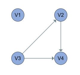
If the query is executed on the graph above, the following vertices will be matched

x	y	z
V1	V2	V4
V1	V3	V2
V1	V3	V4

In that case, three edges will be inserted, one connecting V1 and V2 and two different edges, both connecting V1 and V3 as it is shown below.

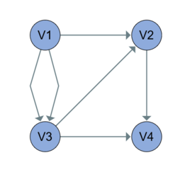
UPDATE

The UPDATE clause allows for setting the properties of one or more vertices and edges.

The syntax is:

UpdateClause       ::= 'UPDATE' GraphElementUpdate ( ',' GraphElementUpdate )*

GraphElementUpdate ::= VariableReference 'SET' '(' PropertyAssignment ( ',' PropertyAssignment )* ')'

For example, the following query sets the property age of every person named “John” to the value 42:

UPDATE x SET ( x.age = 42 )
  FROM MATCH (x:Person)
 WHERE x.name = 'John'

An example in which properties of multiple vertices and edges are update is:

UPDATE v SET ( v.carOwner = true )
     , u SET ( u.weight = 3500 )
     , e SET ( e.since = DATE '2010-01-03' )
  FROM MATCH (v:Person) <-[e:belongs_to]- (u:Car)
 WHERE v.name = 'John'

Above, we match a person named John and the car that belongs to John. We then set the property carOwner of John to true, we set the property weight of the car to 3500, and we set the property since of the belongs_to edge to the date 2010-01-03.

Handling read after write conflicts

During the update, the assigned values (right-hand-side of assignments) correspond to the graph property values before the beginning of the update. This aligns with the snapshot isolation semantics defined between modifications in the same query.

For example consider the following update:

UPDATE x SET ( x.a = y.b, x.b = 12 )
  FROM MATCH (x) -> (y)

It is possible, that a vertex is matched by both (x) and (y) for example

x	y
V1	V2
V3	V1

Supposing that V1.b was 20 before executing the update, V1.b will be assigned 12 V3.a will be assigned 20 no matter in which order the updates are executed.

Handling write after write conflicts

Multiple writes to the same property of the same entity are not allowed, in such cases the execution terminates with an error.

For example consider the following query:

UPDATE x SET ( x.a = y.a )
  FROM MATCH (x) -> (y)

If the following vertices are matched

x	y
V1	V2
V1	V3

a runtime exception will be thrown, because the value assigned to V1.a could be ambiguous.

As an extension to this semantics, PGX implements a more relaxed version for conflicting write checks. If the assigned value can be statically guaranteed to be only depending on property values of the entity it is assigned to, then even in case of multiple assignments, (since the assigned value is always the same) the update succeeds.

For example, in the following case, multiple writes to v.a are allowed, because in this case no matter how many times v.a is written, it is always assigned the same value (65 minus its age property).

UPDATE v SET ( v.a = 65 - v.age )
  FROM MATCH (v:Person) -> (u:Person)
 WHERE v.name = 'John'

In the following case, however, multiple writes to v.a are not allowed, because the value of the property would be ambiguous, 65 minus the other vertex’s age property, that can be different for different matched u’s.

UPDATE v SET ( v.a = 65 - u.age )
  FROM MATCH (v:Person) -> (u:Person)
 WHERE v.name = 'John'

DELETE

DeleteClause ::= 'DELETE' VariableReference ( ',' VariableReference )*

Entities can be deleted by enumerating them after the DELETE keyword. The order of enumeration does not affect the result of the execution.

For example, one can delete all edges from a graph using the following query

DELETE e
  FROM MATCH () -[e]-> ()

Multiple deletes to the same entity are not considered conflicting. For example consider the following query:

DELETE x, y
  FROM MATCH (x) -> (y)

In that case, even if a vertex is matched multiple times by (x) or (y), and deleted multiple times, the query will complete without an exception.

If a vertex is deleted, all its incoming and outgoing edges are deleted as well, thus there are no dangling edges left after a query. So the following query not only deletes the vertex with id 11 but also all edges for which it is source or destination.

DELETE x
  FROM MATCH (x)
 WHERE id(x) = 11

Because of implicit deletion of edges, the following query can be used to delete all edges as well as all vertices from a graph:

DELETE x
  FROM MATCH (x)

Combining INSERT, UPDATE and DELETE

Multiple modifications can be executed in the same query. For example, to update a vertex and also insert an edge with the same vertex as source, the following query can be used:

INSERT EDGE e BETWEEN x AND y
UPDATE y SET ( y.a = 12 )
  FROM MATCH (x), MATCH (y)
 WHERE id(x) = 1 AND id(y) = 2

Isolation semantics of modification queries

Modify queries follow snapshot isolation, which means all modifications see a consistent state of the graph, that is its state before the execution of the update. For this reason, property assignments can come from updated and deleted vertices, but they cannot refer to inserted vertices.

For example, the query below succeeds, because y.age is evaluated based on the graph’s status before the query.

INSERT VERTEX x PROPERTIES ( x.age = y.age )
DELETE y
  FROM MATCH (y)

Please note, that for the same reason, properties of newly inserted vertices cannot be referenced in the right-hand-side expressions. For example, the following query would fail as x is not yet in the graph, and x.age cannot be evaluated:

INSERT VERTEX x PROPERTIES ( v.age = 24 )
     , VERTEX y PROPERTIES ( y.age = x.age )

Handling conflicting modifications

Multiple modifications on the same entity are not allowed, in such cases the execution terminates with an error. This section only addresses conflicts between different modifications under the same query. For the conflicts within the same modification, please refer to the corresponding sections.

One example for such conflict would be the UPDATE-DELETE conflicts. The same entity cannot be updated and deleted in the same query.

For example, let us consider the following query:

UPDATE x SET ( x.a = 11 )
DELETE x
  FROM MATCH (x)

There the conflict is trivial between the deleted and the updated vertex. However, the conflict is not always straightforward, for example, the following query can also fail due to conflicting update and delete:

UPDATE x SET ( x.a = 11 )
DELETE y
  FROM MATCH (x) -> (y)

If the vertices matched by x are distinct to the ones matched by y the query should pass, however, if there is a vertex that is matched by both x and y the query will fail with an exception. Note that the order of modifications does not matter, the query will fail in any case.

Similar behavior is expected upon INSERT-DELETE conflicts, where the inserted entity depends on an entity that is being deleted. Note that because of the snapshot semantics, this is only possible if an edge is inserted, and at the same time its source or destination vertex is deleted.

For example, consider the following, not trivial case:

INSERT EDGE e BETWEEN x AND y
DELETE z
  FROM MATCH (x) -> (y), MATCH (z)
 WHERE id(z) = 11

If any vertex is matched by z and either x or z then after executing the query the inserted edge would not have a source or destination. Thus in that case the execution fails.

Other Syntactic rules

Identifiers

Graph names, property names, labels, etc. are identifiers that can appear in either unquoted form or double quoted form.

The syntax is:

Identifier           ::= UNQUOTED_IDENTIFIER | QUOTED_IDENTIFIER

Unquoted identifiers

Unquoted identifiers take the form of an alphabetic character followed by zero or more alphanumeric or underscore (i.e. _) characters:

UNQUOTED_IDENTIFIER  ::= [a-zA-Z][a-zA-Z0-9\_]*

Unquoted identifiers are automatically uppercased.

For example, the following two queries are equivalent:

SELECT n.dob AS name
  FROM MATCH (n:Person) ON myGraph
 WHERE n.firstName = 'Nikita'

SELECT "N"."DOB"
  FROM MATCH ("N":"PERSON") ON "MYGRAPH"
 WHERE "N"."FIRSTNAME" = 'Nikita'

Note that this is aligned to SQL, which also automatically uppercases unquoted identifiers. However, as an extension to SQL — which matches uppercased references in exact manner — PGQL matches uppercased references to graphs, labels and properties in case-insensitive manner if no exact match exists.

For example, a property firstName in the graph can be referenced in PGQL either through firstName, "firstName", "FIRSTNAME" or fIrStNaMe, but not through "FirstName".

Quoted identifiers

Quoted identifiers are delimited with double quotes and support the full range of Unicode characters:

QUOTED_IDENTIFIER            ::= '"' ( ~[\"] | ESCAPED_IDENTIFIER_CHARACTER )* '"'

ESCAPED_IDENTIFIER_CHARACTER ::= '""'

Above says that a quoted identifier starts and ends with double quotes and in between has any number of:

Unicode characters except for the double quote character
An escaped double quote in the form of two double quotes

Note that the syntax of a PGQL identifier is different from a string literal in languages like Java or C++, because unlike in Java and C++, characters like a new line or a backslash are not escaped in PGQL; in identifiers in PGQL, only double quotes are escaped.

For example, take the following string:

My string with single quotes ', double quotes ", backslashes \
new lines and tabs	.

Here is an example of how to use such a string as a property name in PGQL:

SELECT *
  FROM MATCH (n)
 WHERE n."My string with single quotes ', double quotes "", backslashes \
new lines and tabs	." = 123

As you can see, only the double quote (") was escaped ("").

String literals

The syntax for string literals is:

STRING_LITERAL                   ::= "'" ( ~[\'] | ESCAPED_STRING_LITERAL_CHARACTER )* "'"

ESCAPED_STRING_LITERAL_CHARACTER ::= "''"

Above says that a string literal starts and ends with single quotes and in between has any number of:

Unicode characters except for the single quote character
An escaped single quote in the form of two single quotes

Note that this is different from string literals in languages like Java or C++. First of all, PGQL string literals are single-quoted instead of double-quoted. Second, unlike in Java and C++, characters like a new line or a backslash are not escaped in PGQL; in string literals in PGQL, only single quotes are escaped.

For example, take the following string:

My string with single quotes ', double quotes ", backslashes \
new lines and tabs	.

Here is an example of how to use such a string as literal in PGQL:

SELECT *
  FROM MATCH (n)
 WHERE n.prop = 'My string with single quotes '', double quotes ", backslashes \
new lines and tabs	.'

As you can see, only the single quote (') was escaped ('').

Keywords

The following is a list of keywords in PGQL.

PATH, SELECT, FROM, MATCH, ON, WHERE, GROUP,
BY, HAVING, ORDER, ASC, DESC, LIMIT, OFFSET,
AND, OR, NOT, true, false, IS, NULL, AS,
DATE, TIME, TIMESTAMP, WITH, ZONE, DISTINCT,
COUNT, MIN, MAX, AVG, SUM, ARRAY_AGG, IN,
EXISTS, CAST, CASE, WHEN, THEN, ELSE, END,
EXTRACT, YEAR, MONTH, DAY, HOUR, MINUTE,
SECOND, TIMEZONE_HOUR, TIMEZONE_MINUTE,
TOP, SHORTEST, CHEAPEST, COST, CREATE,
PROPERTY, GRAPH, VERTEX, EDGE, TABLES,
LABEL, PROPERTIES, ARE, ALL, COLUMNS,
EXCEPT, NO, INSERT, UPDATE, DELETE, INTO,
LABELS, SET, BETWEEN

Keywords are case-insensitive and variations such as SELECT, Select and sELeCt can be used interchangeably.

Integers and Decimals

Lexical grammar for integers and decimals is:

UNSIGNED_INTEGER     ::= [0-9]+

UNSIGNED_DECIMAL     ::= ( [0-9]* '.' [0-9]+ ) | ( [0-9]+ '.' )

These rules describe the following:

Unsigned integers consist of one or more digits.
Unsigned decimals either consist of zero or more digits followed by a dot (.) and one or more digits, or, the conceit of one or more digits followed by only a dot (.).

Comments

Comments are delimited by /* and */.

The syntax is:

COMMENT ::= '/*' ~[\*]* '*/'

For example:

/* This is a
   multi-line
   comment. */
SELECT n.name, n.age
  FROM MATCH (n:Person) /* this is a single-line comment */

PGQL 1.3 Specification

Introduction

Changelog

New features in PGQL 1.3

Syntax changes in PGQL 1.3

A note on the Grammar

Document Outline

Property graph data model

Example 1: Student Network

Example 2: Financial Transactions

Creating a Property Graph

CREATE PROPERTY GRAPH

Vertex tables

Edge tables

Table aliases

Keys

Labels

Properties

PROPERTIES ARE ALL COLUMNS

PROPERTIES ARE ALL COLUMNS EXCEPT ( .. )

PROPERTIES ( .. )

NO PROPERTIES

Relation between labels and properties

Source or destination is self

Example: HR schema

Multiple schemas

DROP PROPERTY GRAPH

Graph Pattern Matching

Writing simple queries

Vertex patterns

Edge patterns

Label expressions

Label disjunction

Omitting a label expression

Filter predicates

More complex patterns

Binding an element multiple times

Matching edges in any direction

Main query structure

SELECT

Assigning variable name to Select Expression

SELECT *

FROM

MATCH

ON clause

Default graphs

Querying multiple graphs

Repeated variables

Alternatives for specifying graph patterns

Disconnected graph patterns

Label predicates

WHERE

Grouping and Aggregation

GROUP BY

Multiple Terms in GROUP BY

Aliases in GROUP BY

GROUP BY and NULL values

Repetition of Group Expression in Select or Order Expression

Aggregation

Aggregation with GROUP BY

Aggregation without GROUP BY

COUNT(*)

DISTINCT in aggregation

HAVING

Sorting and Row Limiting

ORDER BY

Data types for ORDER BY

Multiple expressions in ORDER BY

LIMIT and OFFSET

Variable-Length Paths

Quantifiers

Reachability

Examples with various quantifiers

Zero or more

One or more

Optional

Exactly n

n or more

Between n and m

Between zero and m